Brine
A certain person trying to make his way in the universe.
暑假地球科學讀書會
大氣動力學
Presenter: 122527 Brine
Drawing on computer is hard. Have mercy on me.
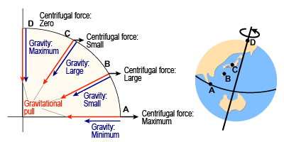
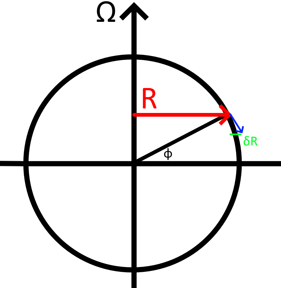
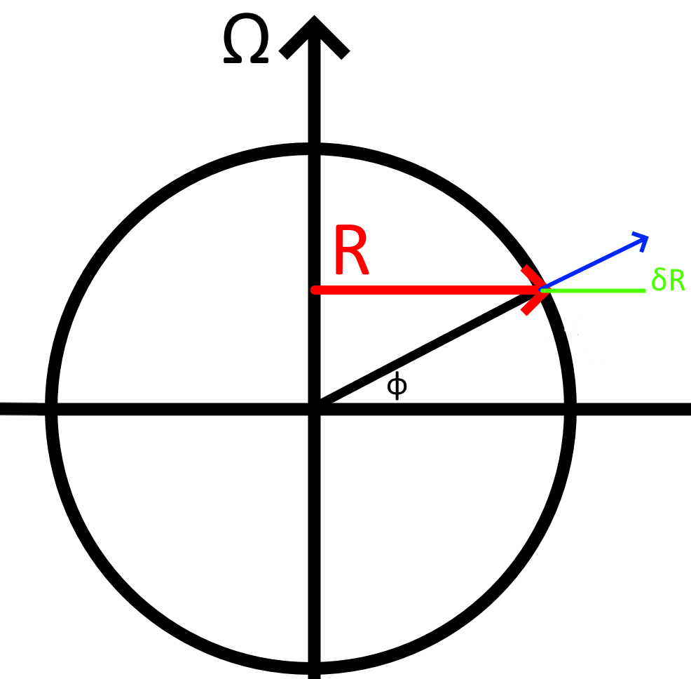
x is parallel to the line of latitude
y is parallel to the line of longitude
z is the altitude
(observed)
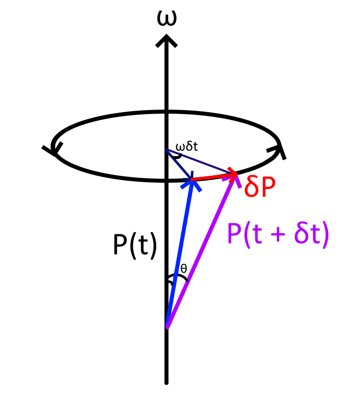
Using simple calculus
Using simple calculus
Using simple calculus
Using simple calculus
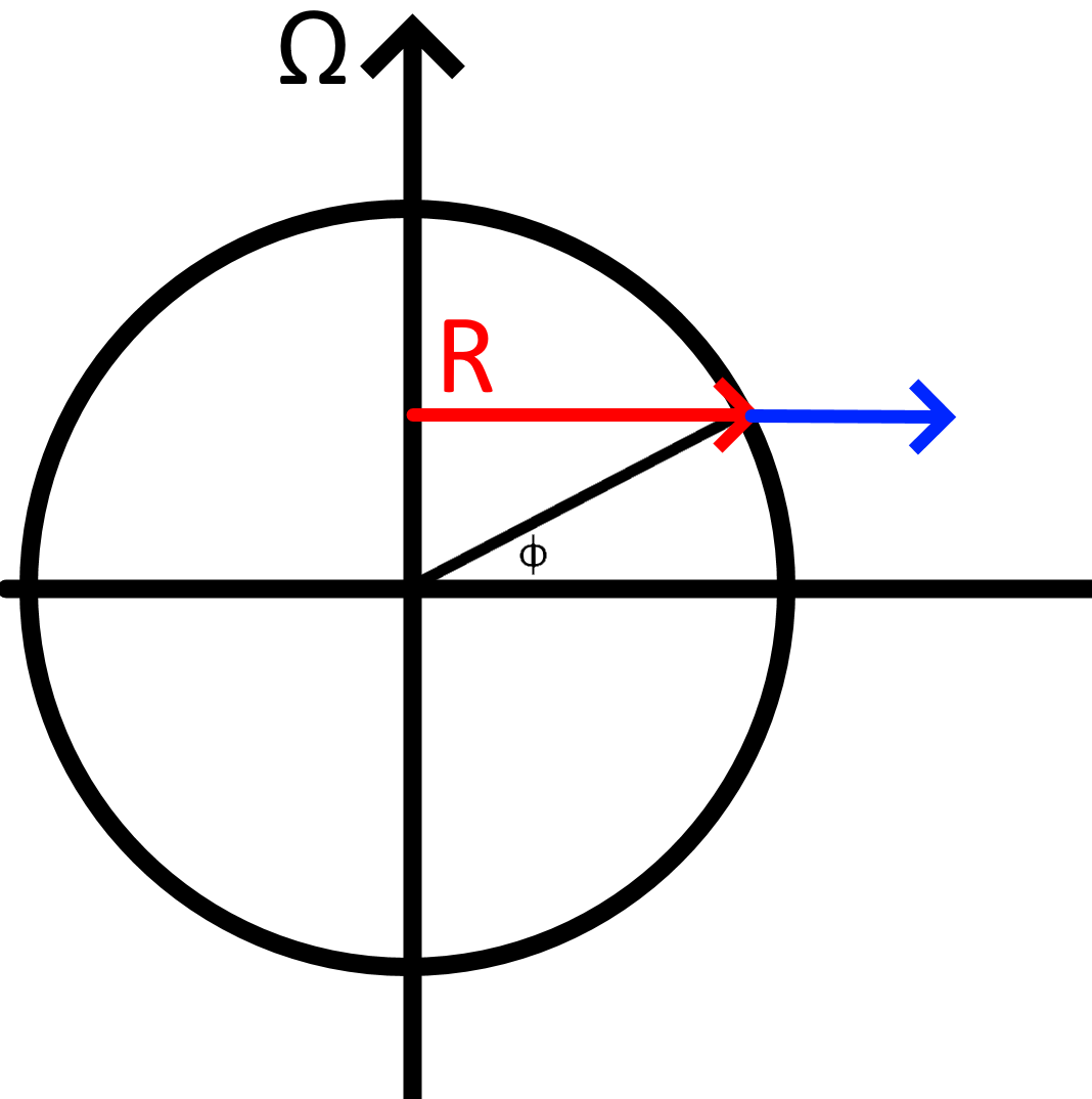
Another approach - u
Another approach - v
Another approach - w
Another approach - conclusion
Another approach - conclusion
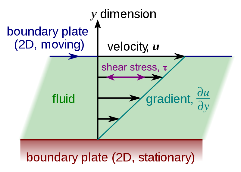
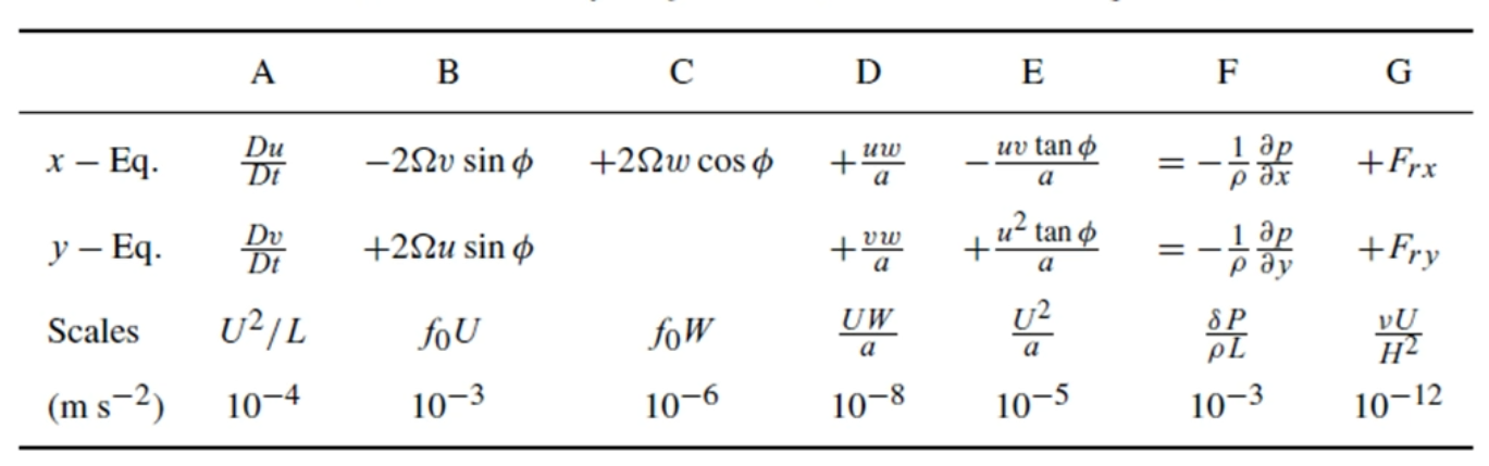
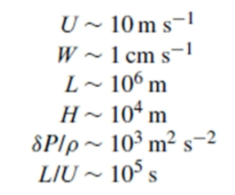
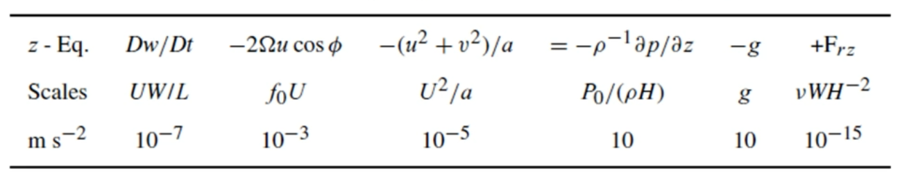
Introduction to some of the equations
What can we do with all of that
I've got nothing left lmao
By Brine
The study of motion systems of meteorological importance, integrating observations at multiple locations and times and theories.


