Adaptive Mesh Refinement Simulations
of Cosmological Scalar Fields
Bodo Schwabe
University of Zaragoza
Scalar Fields in Cosmology

[arXiv: 2110.15109]
[arXiv: 2110.09145]
[in preparation]
[in preparation]
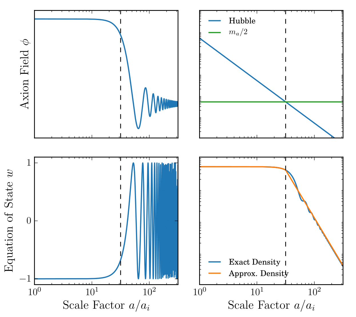
Massive Cosmological Scalar Fields
\ddot{\phi}+3H\dot{\phi}-\nabla^2\phi+m_a^2\phi=0
Axion equation of motion:
Background energy density and pressure:
\overline{\rho}_a=\frac{1}{2}\dot{\phi}^2+\frac{1}{2}m_a^2\phi^2 \\
\overline{P}_a=\frac{1}{2}\dot{\phi}^2-\frac{1}{2}m_a^2\phi^2 \\
\overline{P}_a=\omega_a\overline{\rho}_a
\phi=a^{-3/2}(t/t_i)^{1/2}[C_1J_n(m_at)+C_2Y_n(m_at)]
Solution:
[arXiv:1510.07633]
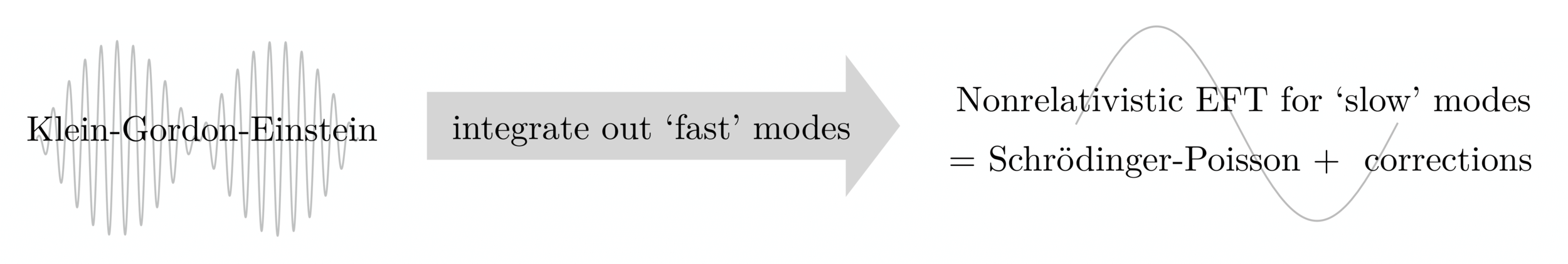
The non-relatistic limit
[arXiv:2104.10128]
\phi = \frac{\hbar}{\sqrt{2}m}\overline{\psi} e^{-imt/\hbar}
i\hbar\partial_{t}\psi = -\frac{\hbar^{2}}{2a^{2}m}\nabla^{2}\psi+mV\psi
\left(g^{\mu\nu}\nabla_{\mu}\nabla_{\nu}-\frac{m^{2}}{\hbar^{2}}\right)\phi = 0
T_{\mu\nu} = \nabla_{\mu}\phi\nabla_{\nu}\phi-\frac{1}{2}g_{\mu\nu}\left(g^{\rho\sigma}\nabla_{\rho}\phi\nabla_{\sigma}\phi+\frac{m^{2}}{\hbar^{2}}\phi\right)
R_{\mu\nu}-\frac{1}{2}g_{\mu\nu}R = 8\pi GT_{\mu\nu}
\nabla^{2}V = 4\pi Ga^{-1}\delta\rho
\delta\rho=|\psi|^{2}
Madelung Transformation - Bohmian Quantum Mechanics
i\hbar\partial_{t}\psi = -\frac{\hbar^{2}}{2a^{2}m}\nabla^{2}\psi+mV\psi
\psi = \sqrt{\rho}e^{iS/\hbar}
\partial_{t}\sqrt{\rho} = -\frac{1}{2ma^{2}}\left[2(\nabla\sqrt{\rho})\cdot(\nabla S)+\sqrt{\rho}\nabla^{2}S\right]
imaginary part
\textbf{v}=\nabla\frac{S}{m}
\partial_{t}\rho+\frac{1}{a^{2}}\nabla\cdot(\rho\textbf{v}) = 0
real part
\partial_{t} S = -\left[\frac{(\nabla S)^{2}}{2a^{2}m}+mV+Q\right]
Q = -\frac{\hbar^{2}}{2ma^{2}}\frac{\nabla^{2}\sqrt{\rho}}{\sqrt{\rho}}
\partial_{t}\textbf{v}+\frac{1}{a^{2}}\textbf{v}\cdot\nabla\textbf{v}+\nabla V+\nabla Q = 0
Euler equations of fluid dynamics + quantum corrections !
Schroedinger-Vlasov correspondence similarly to Ehrenfest theorem implies that massive (m>>H) scalar fields behave like CDM on large scales where gradient energy averages out !
[arXiv:1403.5567]
Linear growth of perturbations
a^{2}\partial_{t}\delta\rho+\rho_{0}\nabla\cdot\textbf{v} = 0
\rho_{0}\partial_{t}\textbf{v}+\rho_{0}\nabla V-\frac{\hbar^{2}}{4m^{2}a^{2}}\nabla\left(\nabla^{2}\delta \rho\right) = 0
Linearize Euler equations:
Take time derivative of the first equation and spatial derivative of the second one, combine and take Fourier transform
\partial_{t}^2\rho_{k}+2H\partial_{t}\rho_{k}+\left(\frac{\hbar^{2}k^{4}}{4m^{2}a^{4}}-4\pi G \rho_0\right)\rho_{k} = 0
Last term vanishes at Jeans scale
k_J=(16 \pi Ga \rho_{0})^{1/4}m^{1/2}
Jeans scale vs. deBroglie wavelength
\lambda_{\rm dB}=2\pi\hbar(mv)^{-1}
\simeq\hbar m^{-1}(G\rho)^{-1/2}r^{-1}
v\simeq r/t_{\text{ff}} = r\sqrt{G\rho}
\lambda_{\rm dB}\equiv r
\lambda_{\rm dB}\simeq r_J
\simeq 66.5 a^{1/4}\left(\frac{\Omega_a h^2}{0.12}\right)^{1/4}\left( \frac{m}{10^{-22}\text{ eV}}\right)^{1/2}\text{ Mpc}^{-1}
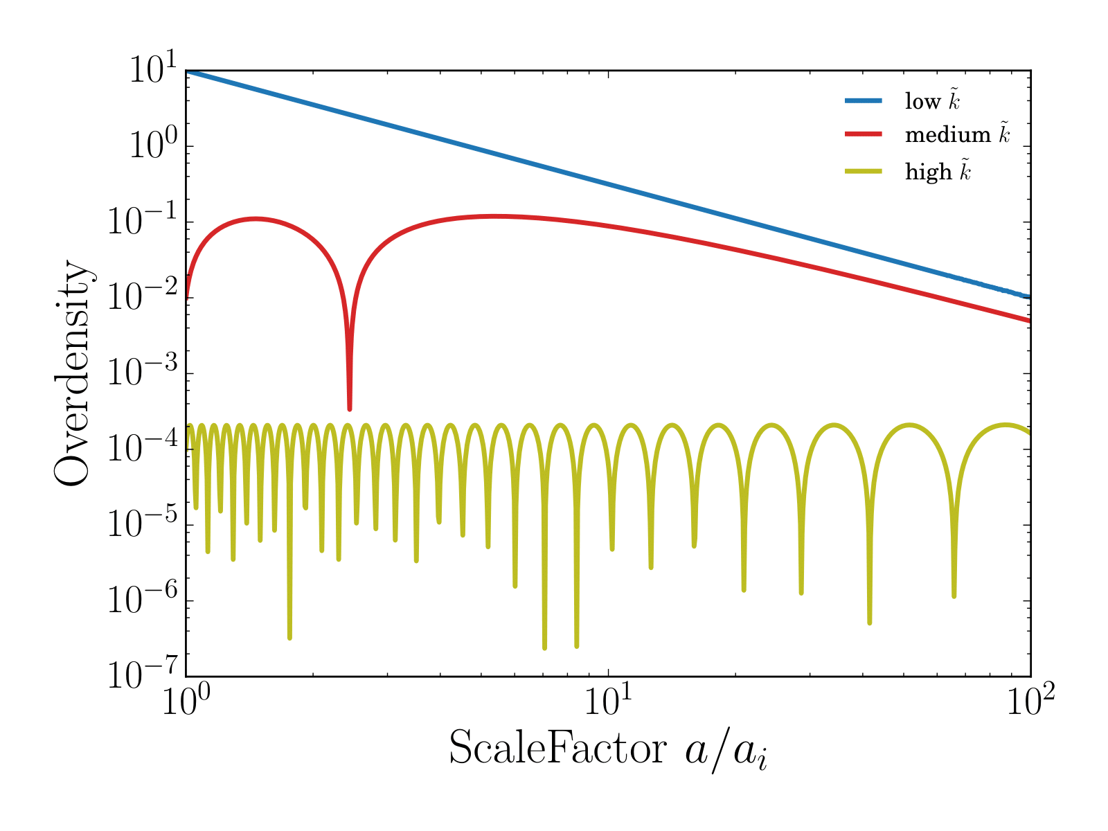
Linear growth of perturbations
\partial_{t}^2\rho_{k}+2H\partial_{t}\rho_{k}+\left(\frac{\hbar^{2}k^{4}}{4m^{2}a^{4}}-4\pi G \rho_0\right)\rho_{k} = 0
\delta_a=C_1 D_+(k,a)+C_2D_-(k,a)
D_+(k,a)= \frac{3\sqrt{a}}{\tilde{k}^2}\sin \left( \frac{\tilde{k}^2}{\sqrt{a}} \right) +\left[ \frac{3a}{\tilde{k}^4}-1 \right]\cos \left( \frac{\tilde{k}^2}{\sqrt{a}} \right)
D_-(k,a)= \left[ \frac{3a}{\tilde{k}^4}-1\right] \sin \left( \frac{\tilde{k}^2}{\sqrt{a}} \right) -\frac{3\sqrt{a}}{\tilde{k}^2}\cos \left( \frac{\tilde{k}^2}{\sqrt{a}} \right)
\tilde{k}=k/\sqrt{m_aH_0}\propto k/k_J
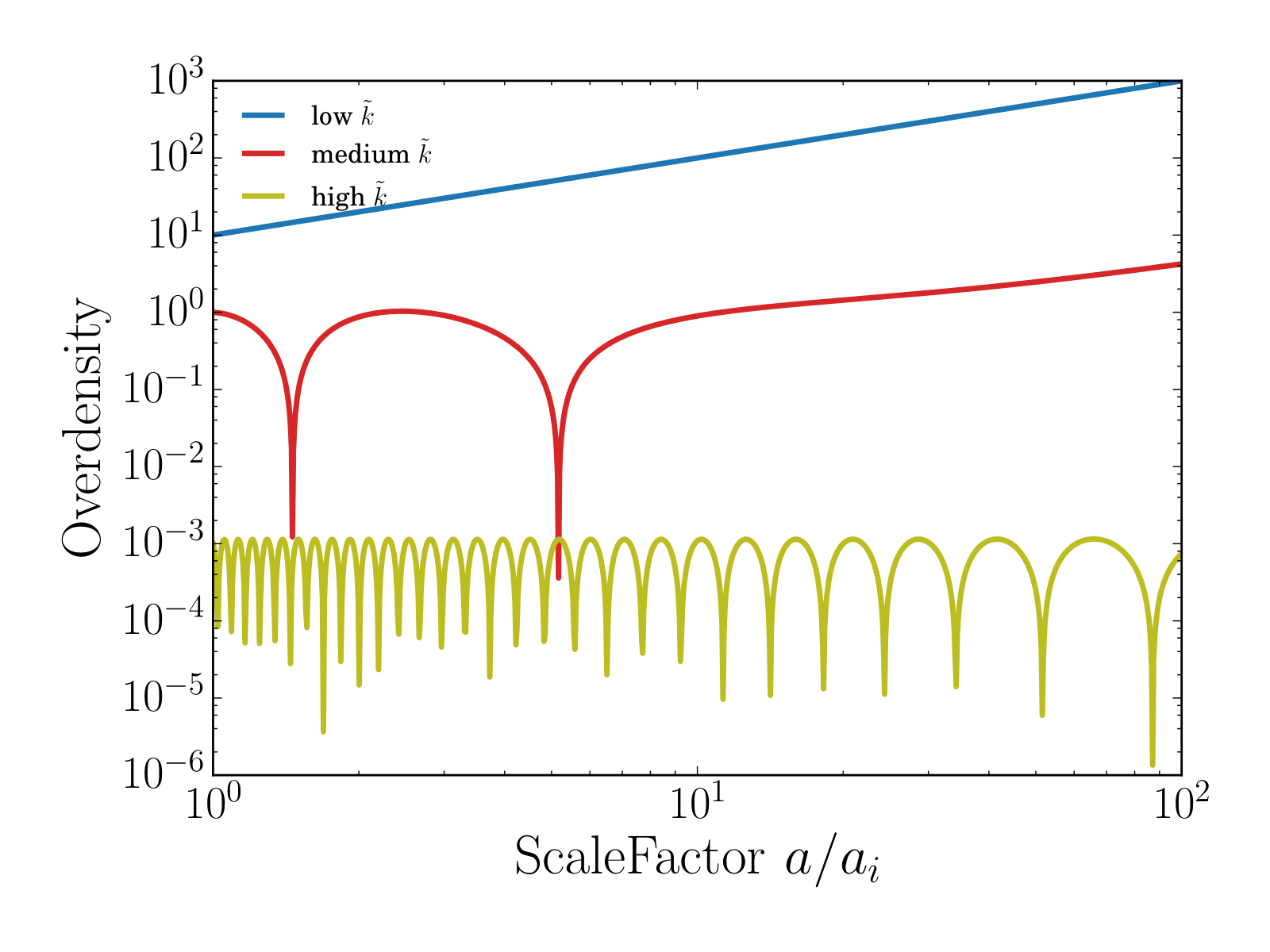
Has exact solution:
,
AxioNyx: Simulating Mixed Fuzzy and Cold Dark Matter
Goal:
- AMR simulations for Mixed Dark Matter
- CDM -> N-body scheme
- FDM -> Spectral/Finite-difference method
- Baryonic physics -> Nyx modules for hydrodynamics and feedback
Bodo Schwabe, Mateja Gosenca, Christoph Behrens, Jens C. Niemeyer, and Richard Easther, Physical Review D, October 2020.
Cosmological Simulations of Mixed Dark Matter
New Hybrid Method
Goal:
- AMR simulation
- Particle method on low resolution levels
- Finite-difference method on finest level
- Important: Boundary conditions between methods
Madelung transformation:
Initial phase:
Phase evolution:
Construction of wavefunction:
Gauss kernel:
\Psi = A\exp[-iSm/\hbar]
\nabla\cdot v_{0} = a^{-1}\nabla^{2} S_{0}
\frac{\text d S_{i}}{\text d t} = \frac{1}{2} {v_i}^2 - V({x_i})
\qquad \Psi({x}) = \sum_i W({x} - {x_i}) A_i e^{i(S_i + {v_i}\cdot a({x}-{x_i}))m/\hbar}
Goal:
- AMR simulation
- Particle method on low resolution levels
- Finite-difference method on finest level
- Important: Boundary conditions between methods
W(x-x_i) = \frac{\gamma^{3/2}\Delta^{3}x}{\pi^{3/2}}\exp\text{[}-\gamma(x-x_i)^{2}\text{]}\theta(x-x_i)
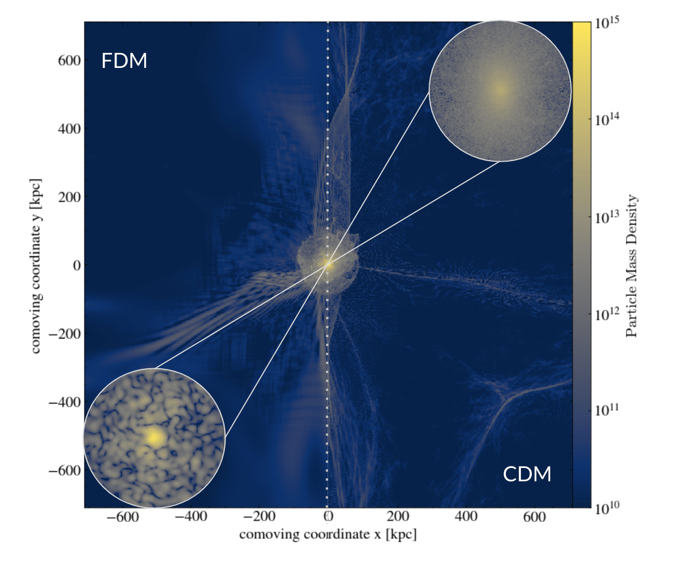
Agora Simulation with FDM
DM-only comparison run (60 Mpc/h) between various codes:
zoom-in simulation focusing on isolated halo


Axionyx N-body run with CDM initial conditions
Axionyx N-body run with FDM initial conditions
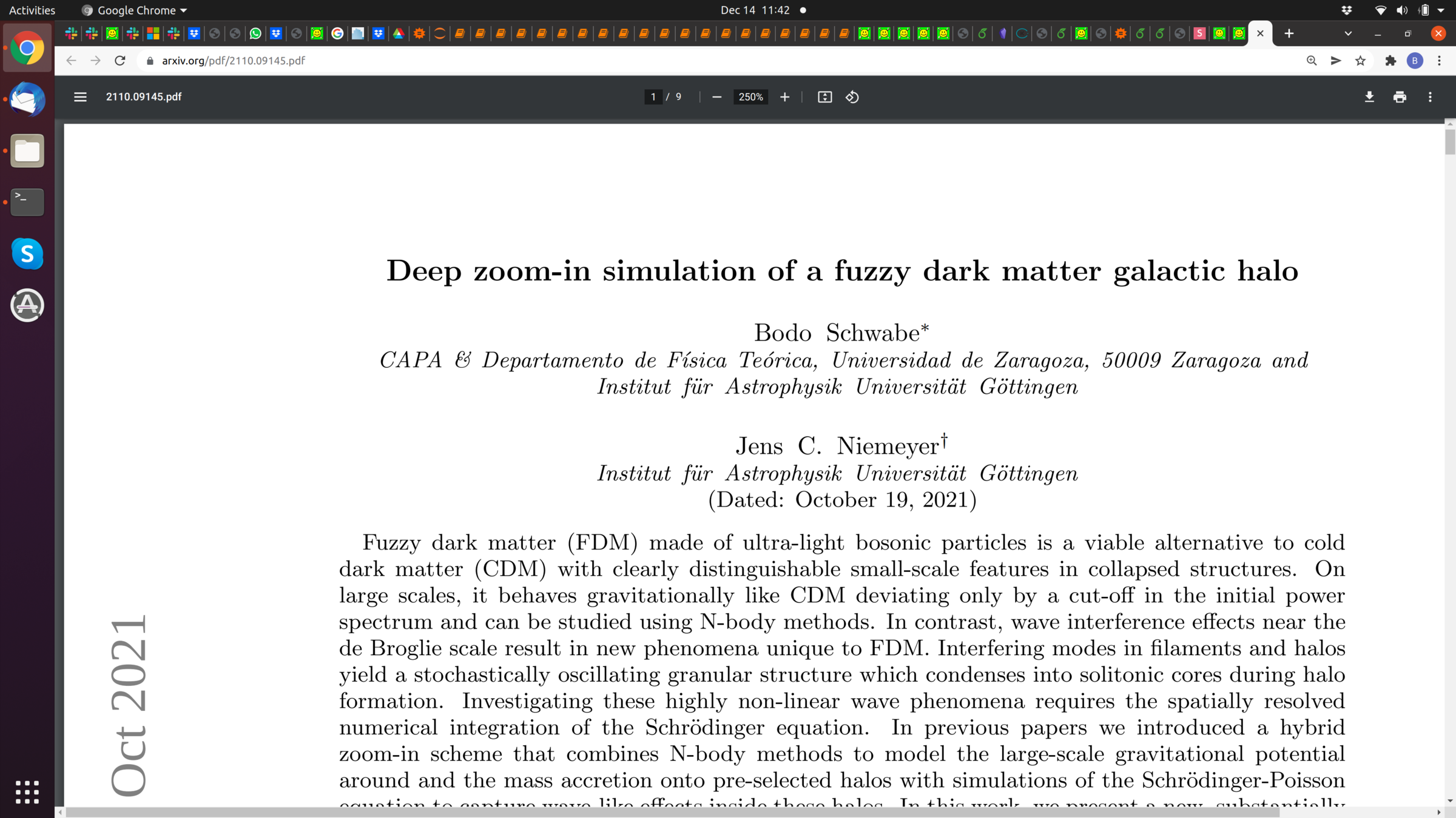
[arXiv: 2110.09145]
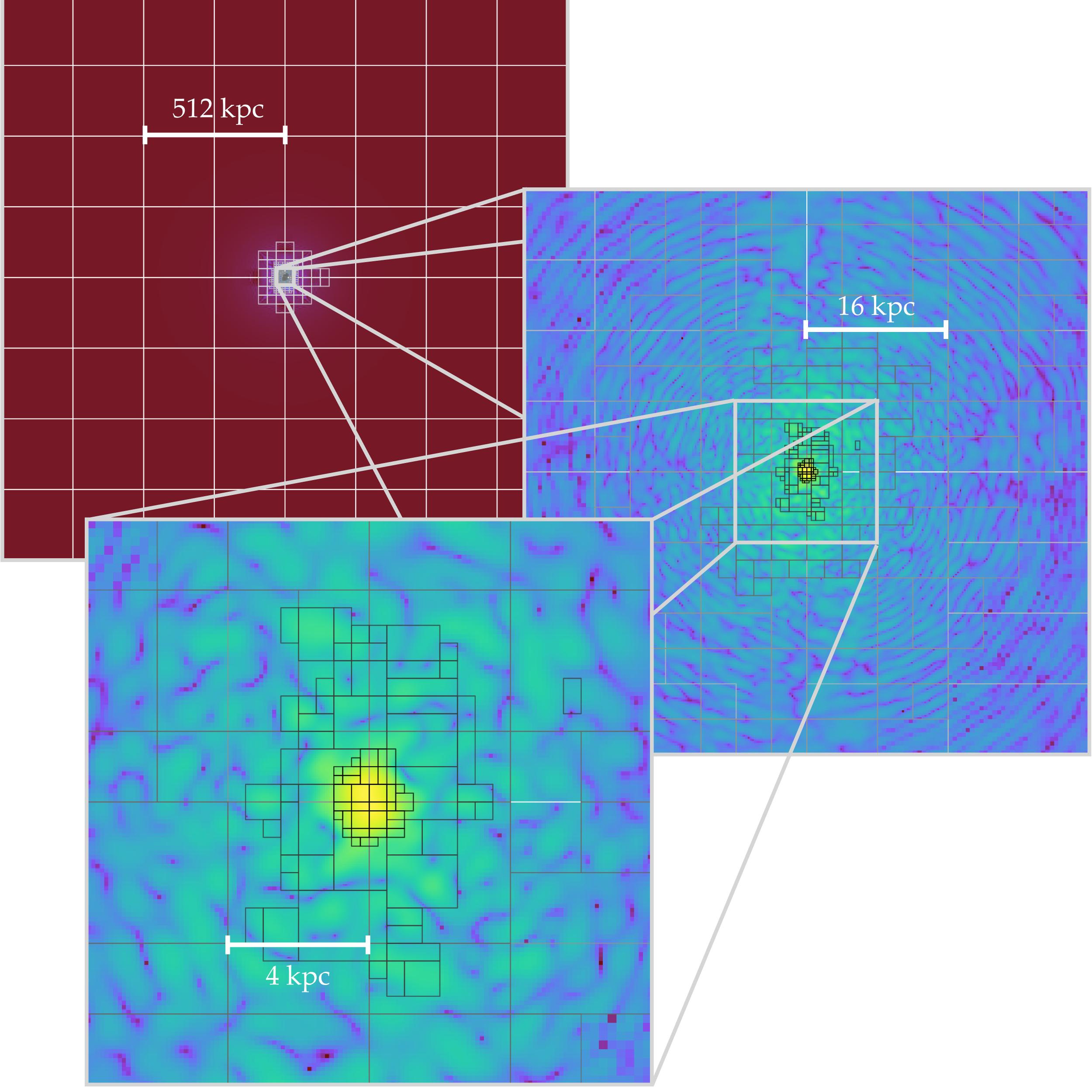
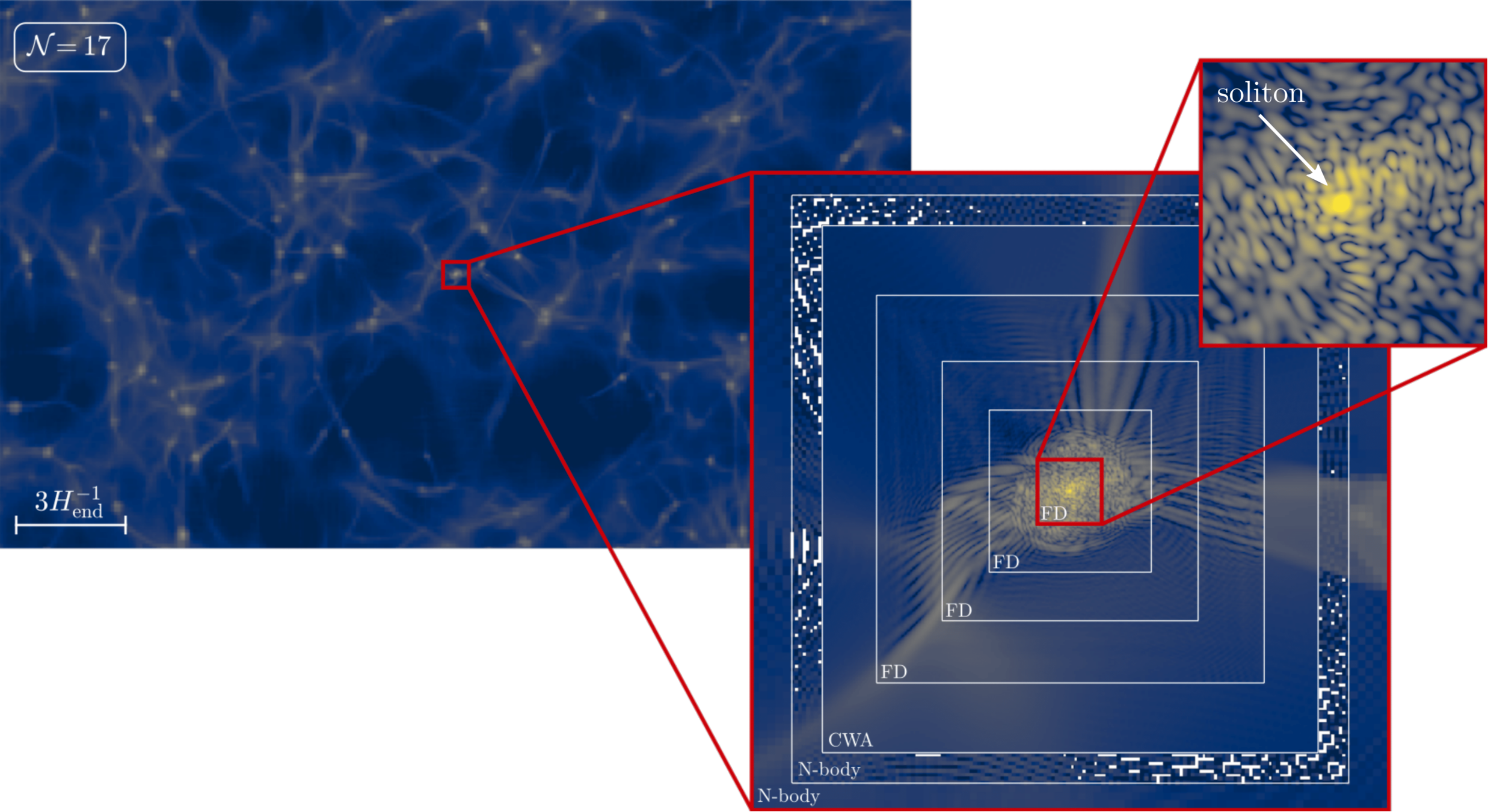
Gauss Beam Reconstruction

- Restart FDM N-body simulation at z=3:
- Reconstruct wavefunction at amr level 11 in the inner most halo region (virial radius at 50kpc)
- Add 3 finite difference levels
The granular structure and central soliton is clearly visible
Agora Simulation


- FDM Powerspectrum and underlying particle velocity dispersion correspond well to each other.
- Halo velocities have not yet relaxed into Maxwell spectrum (but do so later on)
- Soliton velocity (grey line) at peak in spectrum
- FDM radial density profile with soliton core and NFW outer tail
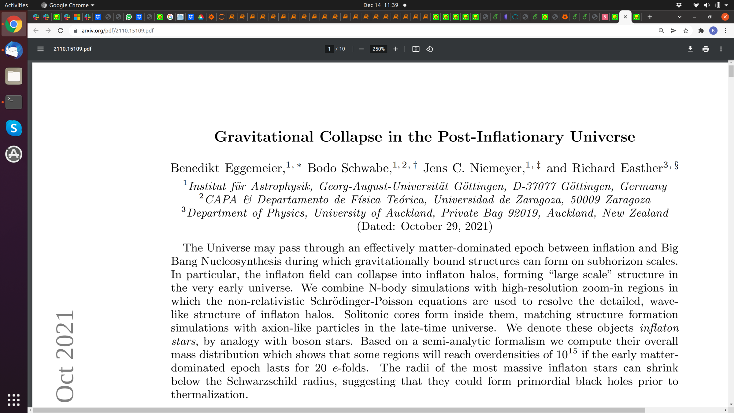
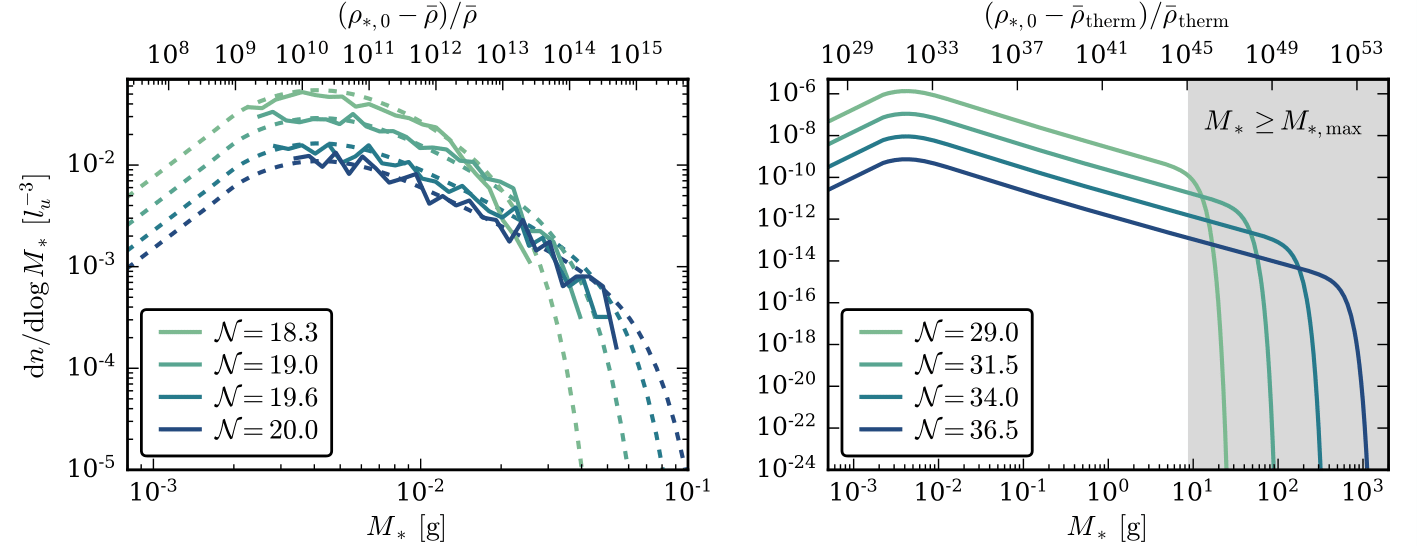
Gravitational Collapse in the Post-Inflationary Universe
- The Universe may pass through an effectively matter-dominated epoch between inflation and Big Bang Nucleosynthesis during which gravitationally bound structures can form on subhorizon scales
- In particular, the inflaton field can collapse into inflaton halos, forming “large scale” structure in the very early universe similar to fuzzy dark matter in late time universe.
[arxiv: 2110.15109]
Gravitational Collapse in the Post-Inflationary Universe
- Mass distribution of inflaton stars shows that some regions will reach overdensities of 10^15 if the early matter-dominated epoch lasts for 20 e-folds. The radii of the most massive inflaton stars can shrink below the Schwarzschild radius, suggesting that they could form primordial black holes prior to thermalization.
KSVZ Axion in Post-Inflationary Scenario
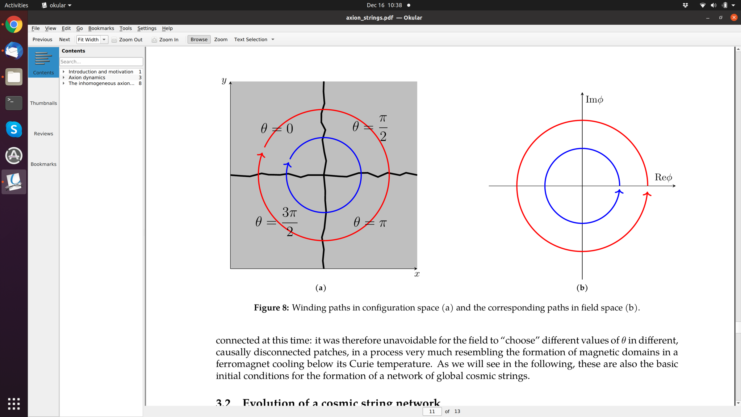
- Random initial axion phases
- PQ-symmetry breaking after inflation
- axion roles down to potential minimum if possible, but topological defects
credit: F. Schiavone
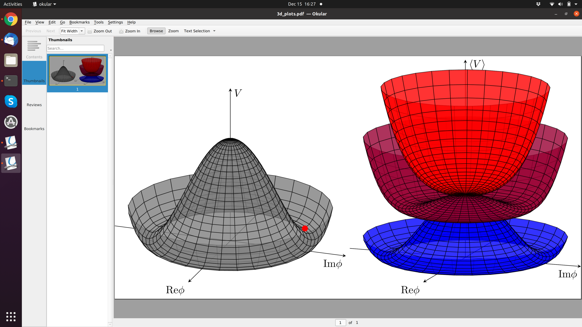
\mathcal{L}_\phi=\frac{1}{2}|\partial_\mu\phi|^2+\lambda(|\phi|^2-v^2)^2+\chi(1-\cos\theta)
\phi=\rho e^{i\theta}


KSVZ Axion in Post-Inflationary Scenario
- Random initial axion phases
- PQ-symmetry breaking after inflation
- axion roles down to potential minimum if possible, but topological defects
credit: F. Schiavone
\mathcal{L}_\phi=\frac{1}{2}|\partial_\mu\phi|^2+\lambda(|\phi|^2-v^2)^2+\chi(1-\cos\theta)


Scale Separation
inter-string separation
string core size
axion decay constant
Hubble scale
10^{30}
- Cosmic expansion increases separation (solution PRS strings)
- not feasible on 3D uniform grids
- possible solution: adaptive mesh refinement around 1D strings (1024^3 root grid and 10 additional levels -> 14 e-folds)

[Drew, Shellard, 2019,arXiv:1910.01718]
Adaptive Mesh Refinement (AMR)
- Tag cells for refinement using string plaquettes [ Leesa Fleury, Guy D. Moore, 2015, arXiv:1509.00026 ]
- create new grids with progressively more resolution on higher levels
- Use MPI communication to transfer interpolated data between grids and levels
- subcycling: use smaller time steps on higher resolved levels
- evolve with spectral method on root grid and finite differencing on higher levels

We extended AxioNyx for AMR string simulations
Use AMR to keep string resolution fixed

[Buschmann et.al. arXiv:2108.05368]


AMR can improve current extrapolations
[Gorghetto et.al., arXiv: 1806.04677, 2007.04990 ]


[Buschmann et.al. arXiv:2108.05368]
[Buschmann et.al. arXiv:2108.05368]
q=1 \rightarrow m_a = 65 \pm 6 \mu eV
AMR can improve current extrapolations
[Gorghetto et.al., arXiv: 1806.04677, 2007.04990 ]
[Buschmann et.al. arXiv:2108.05368]
[Buschmann et.al. arXiv:2108.05368]
q=1 \rightarrow m_a = 65 \pm 6 \mu eV

KSVZ Axion in Post-Inflationary Scenario
- Random initial axion phases
- PQ-symmetry breaking after inflation
- axion roles down to potential minimum if possible, but topological defects
- roughly one string per Hubble patch
- tilt of the Mexican hat potential
- strings annihilate efficiently radiating axions
credit: F. Schiavone
\mathcal{L}_\phi=\frac{1}{2}|\partial_\mu\phi|^2+\lambda(|\phi|^2-v^2)^2+\chi(1-\cos\theta)
KSVZ Axion in Post-String Scenario
- Random initial axion phases
- PQ-symmetry breaking after inflation
- axion roles down to potential minimum if possible, but topological defects
- roughly one string per Hubble patch
- tilt of the Mexican hat potential
- strings annihilate efficiently radiating axions
- What is their final phase space density?
credit: F. Schiavone
\mathcal{L}_\phi=\frac{1}{2}|\partial_\mu\phi|^2+\lambda(|\phi|^2-v^2)^2+\chi(1-\cos\theta)
\mathcal{L}_\theta=\frac{1}{2}|\partial_\mu\theta|^2+\chi(1-\cos\theta)
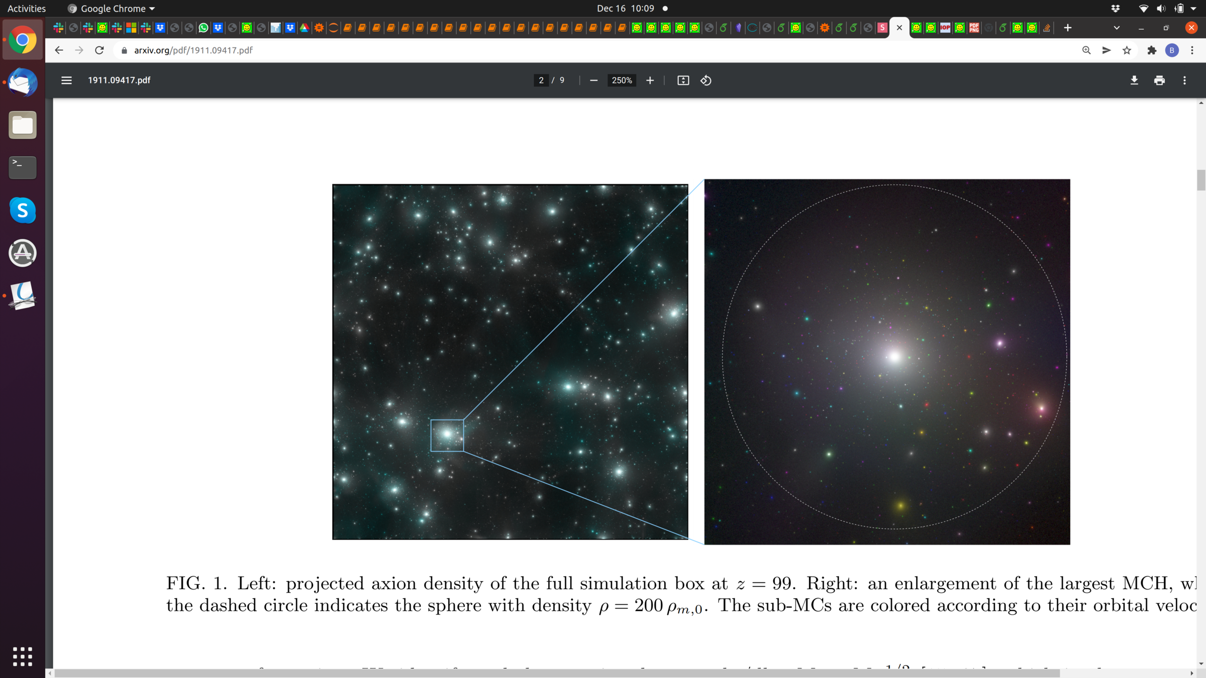
[arXiv: 1911.09417]

¡Muchas Gracias a todos!
Institut talk
By bschwabe


