


Kevin Song
I'm a student at UT (that's the one in Austin) who studies things.
Kevin Song
2024-03-19
Camera View
True System
Camera View
True System
Camera View
True System
Camera View
True System
Camera View
True System
Now that we've just seen a state change on the camera, are we more likely to see the particle continue through, or return to its old state?
Camera View
True System
Now that we've just seen a state change on the camera, are we more likely to see the particle continue through, or return to its old state?
Camera View
True System
Now that we've just seen a state change on the camera, are we more likely to see the particle continue through to the next state, or return to the old state?
Continue through
Camera View
True System
Now that we've just seen a state change on the camera, are we more likely to see the particle continue through to the next state, or return to the old state?
Continue through
Return
Camera View
True System
Now that we've just seen a state change on the camera, are we more likely to see the particle continue through to the next state, or return to the old state?
Continue through
Return
Appears that particle remembers its old state!
Can be mathematically described by a stochastic process.
A set of random variables indexed by a time variable \(i \in \mathcal{T}\), with outcome space \(\mathcal{X}\)
TIME
The next state of the stochastic process depends on the previous \(n\) values, but nothing more.
Important note: if \(n \geq 2\), the process is considered "non-Markov"
Writing out the names of all the random variables and the outcomes leads to a lot of visual noise.
We will often use just the lowercase outcome names and implicitly use them as the outcome of the random variable with the same uppercase name.
If we use empirical probabilities, the equality will rarely ever be satisfied for the same reason that tossing 100 coins rarely results in 50 heads and 50 tails.
(2) Sokolov, Igor M. 2012. “Models of Anomalous Diffusion in Crowded Environments.” Soft Matter 8 (35): 9043–52.
Metzler, Ralf, and Joseph Klafter. 2000. “The Random Walk’s Guide to Anomalous Diffusion: A Fractional Dynamics Approach.” Physics Reports 339 (1): 1–77.
Muñoz-Gil, Gorka, Giovanni Volpe, Miguel Angel Garcia-March, Erez Aghion, Aykut Argun, Chang Beom Hong, Tom Bland, et al. 2021. “Objective Comparison of Methods to Decode Anomalous Diffusion.” Nature Communications 12 (1): 6253.
(1) Dudko, Olga K., Gerhard Hummer, and Attila Szabo. 2006. “Intrinsic Rates and Activation Free Energies from Single-Molecule Pulling Experiments.” Physical Review Letters 96 (10): 108101.
Dudko, Olga K., Gerhard Hummer, and Attila Szabo. 2008. “Theory, Analysis, and Interpretation of Single-Molecule Force Spectroscopy Experiments.” Proceedings of the National Academy of Sciences of the United States of America 105 (41): 15755–60.
Best, Robert B., and Gerhard Hummer. 2011. “Diffusion Models of Protein Folding.” Physical Chemistry Chemical Physics: PCCP 13 (38): 16902–11.
(side note: this never happens)
Berezhkovskii, Alexander M., and Dmitrii E. Makarov. 2018. “Single-Molecule Test for Markovianity of the Dynamics along a Reaction Coordinate.” Journal of Physical Chemistry Letters 9 (9): 2190–95.
Berezhkovskii, Alexander M., and Dmitrii E. Makarov. 2018. “Single-Molecule Test for Markovianity of the Dynamics along a Reaction Coordinate.” Journal of Physical Chemistry Letters 9 (9): 2190–95.
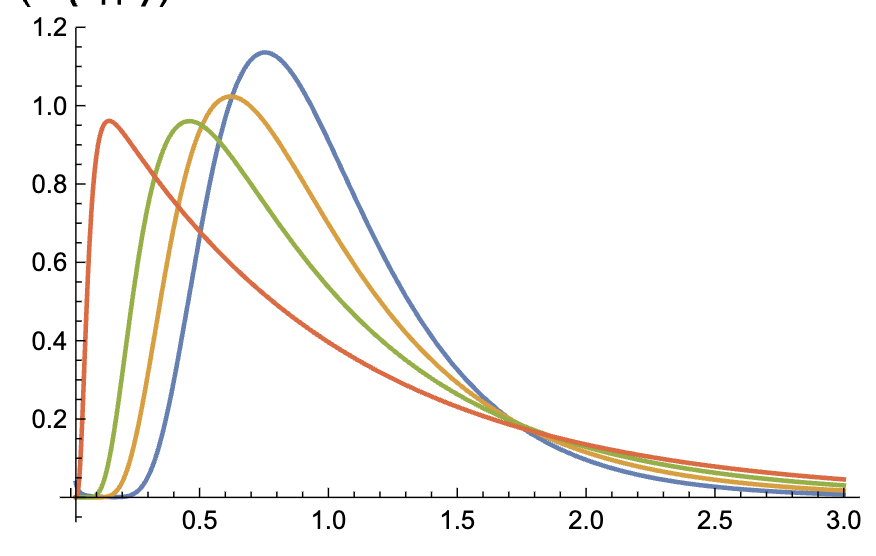
How wide can the distribution of transition path times be?
If they're wider than a certain cutoff, the dynamics result from projection of multidimensional dynamics onto 1D.
Satija, Rohit, Alexander M. Berezhkovskii, and Dmitrii E. Makarov. 2020. “Broad Distributions of Transition-Path Times Are Fingerprints of Multidimensionality of the Underlying Free Energy Landscapes.” Proceedings of the National Academy of Sciences of the United States of America 117 (44): 27116–23.
Transition Path (TP) Time
Probability of TP Time
(1) Zijlstra, Niels, Daniel Nettels, Rohit Satija, Dmitrii E. Makarov, and Benjamin Schuler. 2020. “Transition Path Dynamics of a Dielectric Particle in a Bistable Optical Trap.” Physical Review Letters 125 (14): 146001.
(2) Makarov, Dmitrii E. 2021. “Barrier Crossing Dynamics from Single-Molecule Measurements.” The Journal of Physical Chemistry. B 125 (10): 2467–76.
(3) Lapolla, Alessio, and Aljaž Godec. 2021. “Toolbox for Quantifying Memory in Dynamics along Reaction Coordinates.” Physical Review Research 3 (2): L022018.
"How hard is it to guess the next symbol?"
Easy (low entropy)
Hard (high entropy)
Let's say we repeat this process \(N\) times. How many bits do we need to send over the wire?
Let's say we repeat this process \(N\) times. How many bits do we need to send over the wire?
Shannon's source coding theorem
\( H(X) \) bits per observation
The source coding theorem assumes that the variables occur i.i.d. But this is typically not the case in practice!
The source coding theorem assumes that the variables occur i.i.d. But this is typically not the case in practice!
The source coding theorem assumes that the variables occur i.i.d. But this is typically not the case in practice!
Suppose \( \{X_i\}\) is a Markov process of order \(n\), i.e. an \(n\)-Markov process).
Suppose \( \{X_i\}\) is a Markov process of order \(n\), i.e. an \(n\)-Markov process).
Suppose \( \{X_i\}\) is a Markov process of order \(n\), i.e. an \(n\)-Markov process).
Suppose \( \{X_i\}\) is a Markov process of order \(n\), i.e. an \(n\)-Markov process).
Suppose \( \{X_i\}\) is a Markov process of order \(n\), i.e. an \(n\)-Markov process).
Suppose \( \{X_i\}\) is a Markov process of order \(n\), i.e. an \(n\)-Markov process).
Suppose \( \{X_i\}\) is a Markov process of order \(n\), i.e. an \(n\)-Markov process).
Suppose \( \{X_i\}\) is a Markov process of order \(n\), i.e. an \(n\)-Markov process).
for \(k > n\)
for an \(n\)-Markov process for \(k > n\)
To evaluate the formula for \(h^{(k)}\), we need probabilities of seeing \(k\)-grams and \(k+1\)-grams.
Use empirical frequencies as a proxy for these probabilities.
1 2 2
1
1 2 2
1
2 2 1
1
1 2 2
1
2 2 1
1
2 1 2
1
1 2 2
1
2 2 1
1
2 1 2
1
1 2 1
1
1 2 2
1
2 2 1
1
2 1 2
2
1 2 1
1
1 2 2
1
2 2 1
4
2 1 2
2
1 2 1
3
etc.
etc.
1 2 2
2 2 1
2 1 2
1 2 1
etc.
etc.
1 2 2 1
1
1
4
2
3
1 2 2
2 2 1
2 1 2
1 2 1
etc.
etc.
1 2 2 1
1
2 2 1 2
1
1
4
2
3
1 2 2
2 2 1
2 1 2
1 2 1
etc.
etc.
1 2 2 1
2
2 2 1 2
1
and so on
and so forth
1
4
2
3
1 2 2
2 2 1
2 1 2
1 2 1
etc.
etc.
1 2 2 1
2
2 2 1 2
1
and so on
and so forth
1
4
2
3
1 2 2
1
2 2 1
4
2 1 2
2
1 2 1
3
1 2 2 1
2
2 2 1 2
1
1/37
4/37
2/37
3/37
2/38
1/38
Dębowski, Łukasz. 2016. “Consistency of the Plug-in Estimator of the Entropy Rate for Ergodic Processes.” In 2016 IEEE International Symposium on Information Theory (ISIT), 1651–55. IEEE.
We need at least \(2^{k H(X)}\) points to get an correct estimator of \(h^{k}\).
If we use plug-in estimators, we can always conclude a process is non-Markov. Just pick a large enough \(k\).
Plug-in estimators work well here!
The minimum number of bits needed to communicate a new observation of \(X_i\) given the complete history of \(X_i\) so far.
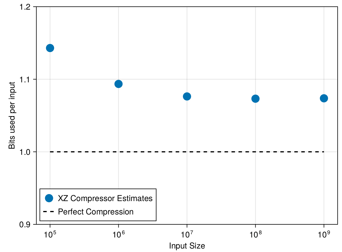
Compression algorithms seem to be a good candidate for estimating this value:
Plug-in estimators work well here!
Compression works well here!
Plug-in estimators work well here!
Compression works well here!
What about here?
LZ77-family algorithms have \(O\left(\frac{\log \log N}{\log N}\right)\) convergence.
Convergence to small error not possible with any reasonable data size.
Song, Kevin, Dmitrii E. Makarov, and Etienne Vouga. 2023. “Compression Algorithms Reveal Memory Effects and Static Disorder in Single-Molecule Trajectories.” Physical Review Research 5 (1): L012026.
Errors in the compression algorithm are empirically strongly dependent on the size of the input, and weakly dependent on the distribution.
Errors in the compression algorithm are empirically strongly dependent on the size of the input, and weakly dependent on the distribution.
Artificially generate a process which has the is known to be \(k\)-Markov, and compare it to the true (observed) process.
| Term | Frequency | Probability |
|---|---|---|
| ... | ... | ... |
| ... | ... | ... |
Pick
\(k\)
Resample k-Markov process
Compress
Compress
=
?
Details here
\(h^{(1)}\) estimated by compression
\(h^{(1)}\) estimated by plug-in method. Can assume this is very accurate.
\(h^{(1)}\) estimated by compression
The error in \(\tilde{h}^{(1)}\).
Also the error in all the compressor estimates, since increasing \(k\) does not shift the error!
The error in \(\tilde{h}^{(1)}\).
The error in \(\tilde{h}^{(k)}\)?
The compressor estimate of \(h^{(k)}\).
The error in \(\tilde{h}^{(k)}\)?
The exact \(k\)th order entropy?
The exact \(k\)th order entropy?
Well....not always. But it comes out pretty close most of the time!
Second order entropy equal to infinite order establishes this is a 2nd order process.
Second order entropy equal to infinite order establishes this is a 2nd order process.
Correctly replicating theoretical entropy rates is an added bonus!
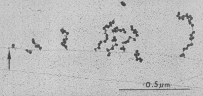
Miller OL Jr, Hamkalo BA, Thomas CA Jr. Visualization of bacterial genes in action. Science. 1970 Jul 24;169(3943):392-5. doi: 10.1126/science.169.3943.392. PMID: 4915822.
Abbondanzieri, Elio A., William J. Greenleaf, Joshua W. Shaevitz, Robert Landick, and Steven M. Block. 2005. “Direct Observation of Base-Pair Stepping by RNA Polymerase.” Nature 438 (7067): 460–65.
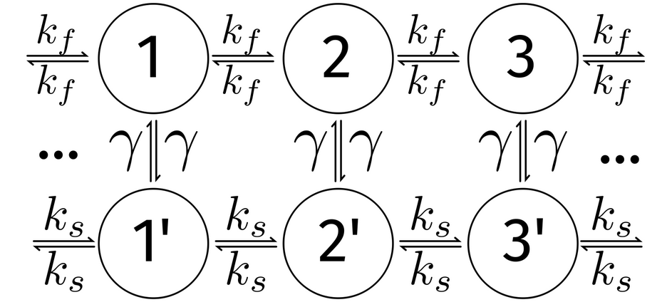
No theoretical results in most regimes of \( \gamma \).
In the limit of high \( \gamma \), should be a Markov process.
In the limit of low \( \gamma \), should recover a half-slow, half-fast walk.
See chapter 4 of the proposal for:
There exist continuous analogues of the entropy, e.g. the differential entropy, which is defined as
Has some weird behaviors. For example, can go to negative infinity for a narrow Gaussian.
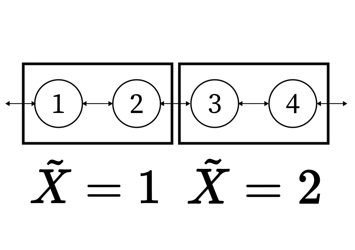
Partition the space into disjoint regions and number them \(\{1 \dots N\}\).
Instead of describing the particle by its \((x, y)\) coordinates, describe it by a number that says which rectangle it's in.
Partition the space into disjoint regions and number them \(\{1 \dots N\}\).
Instead of describing the particle by its \((x, y)\) coordinates, describe it by a number that says which rectangle it's in.
TIME
Milestone
Lump
A
Faradjian, Anton K., and Ron Elber. 2004. “Computing Time Scales from Reaction Coordinates by Milestoning.” The Journal of Chemical Physics 120 (23): 10880–89.
TIME
Milestone
Lump
A
B
1
Faradjian, Anton K., and Ron Elber. 2004. “Computing Time Scales from Reaction Coordinates by Milestoning.” The Journal of Chemical Physics 120 (23): 10880–89.
Faradjian, Anton K., and Ron Elber. 2004. “Computing Time Scales from Reaction Coordinates by Milestoning.” The Journal of Chemical Physics 120 (23): 10880–89.
TIME
Milestone
Lump
A
B
1
A
Faradjian, Anton K., and Ron Elber. 2004. “Computing Time Scales from Reaction Coordinates by Milestoning.” The Journal of Chemical Physics 120 (23): 10880–89.
TIME
Milestone
Lump
A
B
1
A
B
Faradjian, Anton K., and Ron Elber. 2004. “Computing Time Scales from Reaction Coordinates by Milestoning.” The Journal of Chemical Physics 120 (23): 10880–89.
TIME
Milestone
Lump
A
B
1
A
B
C
2
Faradjian, Anton K., and Ron Elber. 2004. “Computing Time Scales from Reaction Coordinates by Milestoning.” The Journal of Chemical Physics 120 (23): 10880–89.
TIME
Milestone
Lump
A
B
1
A
B
C
2
B
Faradjian, Anton K., and Ron Elber. 2004. “Computing Time Scales from Reaction Coordinates by Milestoning.” The Journal of Chemical Physics 120 (23): 10880–89.
TIME
Milestone
Lump
A
B
1
A
B
C
2
B
A
1
Faradjian, Anton K., and Ron Elber. 2004. “Computing Time Scales from Reaction Coordinates by Milestoning.” The Journal of Chemical Physics 120 (23): 10880–89.
TIME
Milestone
Lump
A
B
1
A
B
C
2
B
A
1
B
Faradjian, Anton K., and Ron Elber. 2004. “Computing Time Scales from Reaction Coordinates by Milestoning.” The Journal of Chemical Physics 120 (23): 10880–89.
TIME
Milestone
Lump
A
B
1
A
B
C
2
B
A
1
B
C
2
Faradjian, Anton K., and Ron Elber. 2004. “Computing Time Scales from Reaction Coordinates by Milestoning.” The Journal of Chemical Physics 120 (23): 10880–89.
TIME
Milestone
Lump
A
B
1
A
B
C
2
B
A
1
B
C
2
D
3
Faradjian, Anton K., and Ron Elber. 2004. “Computing Time Scales from Reaction Coordinates by Milestoning.” The Journal of Chemical Physics 120 (23): 10880–89.
TIME
Milestone
Lump
A
B
1
A
B
C
2
B
A
1
B
C
2
D
3
Faradjian, Anton K., and Ron Elber. 2004. “Computing Time Scales from Reaction Coordinates by Milestoning.” The Journal of Chemical Physics 120 (23): 10880–89.
Milestone
Lump
A
B
1
A
B
C
2
B
A
1
B
C
2
D
3
Milestone
Lump
A
B
1
A
B
C
2
B
A
1
B
C
2
D
3
Apply tiny \(\delta t\)
Song, Kevin, Dmitrii E. Makarov, and Etienne Vouga. 2023. “The Effect of Time Resolution on the Observed First Passage Times in Diffusive Dynamics.” The Journal of Chemical Physics 158 (11): 111101.
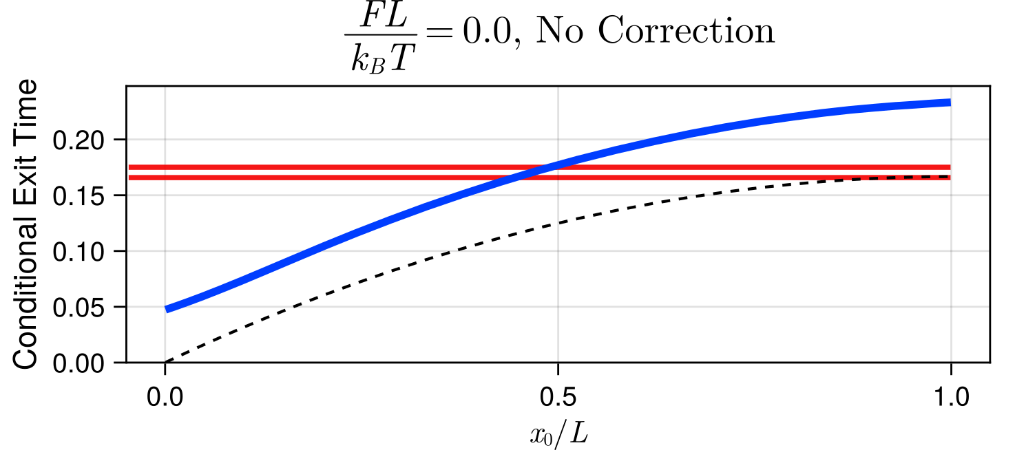
Suppose I am watching a particle diffusing starting from a point \(x = x_0\) and want to know how long it takes the particle to first cross \(x = x_0 + L\).
TIME
For a given time resolution \(\delta t\), how large can the error in this crossing time \( \Delta \) be?
Suppose I am watching a particle diffusing starting from a point \(x = x_0\) and want to know how long it takes the particle to first cross \(x = x_0 + L\).
TIME
For a given time resolution \(\delta t\), how large can the error in this crossing time \( \Delta \) be?
Suppose I am watching a particle diffusing starting from a point \(x = x_0\) and want to know how long it takes the particle to first cross \(x = x_0 + L\).
TIME
For a given time resolution \(\delta t\), how large can the error in this crossing time \( \Delta \) be?
Suppose I am watching a particle diffusing starting from a point \(x = x_0\) and want to know how long it takes the particle to first cross \(x = x_0 + L\).
TIME
For a given time resolution \(\delta t\), how large can the error in this crossing time \( \Delta \) be?
Suppose I am watching a particle diffusing starting from a point \(x = x_0\) and want to know how long it takes the particle to first cross \(x = x_0 + L\).
TIME
For a given time resolution \(\delta t\), how large can the error in this crossing time \( \Delta \) be?
Suppose I am watching a particle diffusing starting from a point \(x = x_0\) and want to know how long it takes the particle to first cross \(x = x_0 + L\).
TIME
For a given time resolution \(\delta t\), how large can the error in this crossing time \( \Delta \) be?
Suppose I am watching a particle diffusing starting from a point \(x = x_0\) and want to know how long it takes the particle to first cross \(x = x_0 + L\).
TIME
For a given time resolution \(\delta t\), how large can the error in this crossing time \( \Delta \) be?
Suppose I am watching a particle diffusing starting from a point \(x = x_0\) and want to know how long it takes the particle to first cross \(x = x_0 + L\).
TIME
For a given time resolution \(\delta t\), how large can the error in this crossing time \( \Delta \) be?
Suppose I am watching a particle diffusing starting from a point \(x = x_0\) and want to know how long it takes the particle to first cross \(x = x_0 + L\).
For a given time resolution \(\delta t\), how large can the error in this crossing time \( \Delta \) be?
TIME
Suppose I am watching a particle diffusing starting from a point \(x = x_0\) and want to know how long it takes the particle to first cross \(x = x_0 + L\).
TIME
For a given time resolution \(\delta t\), how large can the error in this crossing time \( \Delta \) be?
Suppose I am watching a particle diffusing starting from a point \(x = x_0\) and want to know how long it takes the particle to first cross \(x = x_0 + L\).
TIME
For a given time resolution \(\delta t\), how large can the error in this crossing time \( \Delta \) be?
TIME
For a given time resolution \(\delta t\), how large can the error in this crossing time \( \Delta \) be?
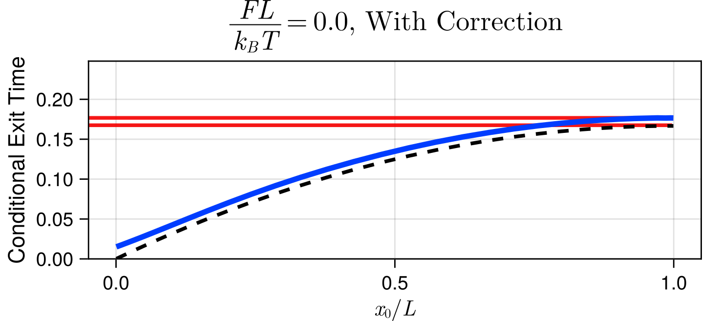
We can explicitly compute the probability that a crossing went unobserved in a timestep based on the positions at the end of each timestep, and reintroduce crossings in a probabilistic manner.
Estimated Mean Exit Time at \(\delta t = 0.01\)
True Mean Exit Time at \(\delta t = 0.01\)
Visualization of \(\delta t = 0.01\)
Estimated Mean Exit Time at \(\delta t = 0.01\)
True Mean Exit Time at \(\delta t = 0.01\)
Visualization of \(\delta t = 0.01\)
Song, Kevin, Raymond Park, Atanu Das, Dmitrii E. Makarov, and Etienne Vouga. 2023. “Non-Markov Models of Single-Molecule Dynamics from Information-Theoretical Analysis of Trajectories.” The Journal of Chemical Physics 159 (6). https://doi.org/10.1063/5.0158930.
Diffusive Simulation, Compression
Diffusive Simulation, Plug-in
Gly-Ser Simulation, Compression
Gly-Ser Simulation, Plug-in
See Chapter 5 of the proposal for:
See Chapter 6 of the proposal for:
Chapter 5: Missed Crossing Correction
Chapter 6: Continuous Markovanity Detection
A: This is a can of worms that I refuse to touch.
A: For the purposes of this section, we'll say something is alive if its actions are not time reversible.
This does have the unfortunate side effect of making things like fires and powerplants alive. ¯\_(ツ)_/¯
It has long been understood that irreversible processes increase the entropy of the universe ("generate entropy").
It was not until recently that this was linked to statements about microscopic trajectories.
Crooks, G. E. 1999. “Entropy Production Fluctuation Theorem and the Nonequilibrium Work Relation for Free Energy Differences.” Physical Review. E, Statistical Physics, Plasmas, Fluids, and Related Interdisciplinary Topics 60 (3): 2721–26.
Average change in entropy over time, averaged over the trajectory
Average change in entropy over time, averaged over the trajectory
Kullback-Leibler Divergence
Average change in entropy over time, averaged over the trajectory
Kullback-Leibler Divergence
Time-reversed version of \(X_t\)
👀
Do the same sorts of problems with estimating entropy rate (inadequate spatial/temporal resolution, issues with coarse-graining) come into play when estimating entropy production?
TIME
1
2
3
Forward Milestone
TIME
1
2
3
Milestone
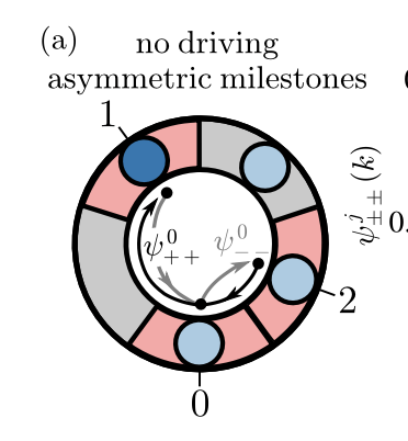
Reverse-then-Milestone
Different waiting times will result in different entropy production!
Hartich, David, and Aljaž Godec. 2023. “Violation of Local Detailed Balance upon Lumping despite a Clear Timescale Separation.” Physical Review Research 5 (3): L032017.
Hartich, David, and Aljaž Godec. 2021. “Emergent Memory and Kinetic Hysteresis in Strongly Driven Networks.” Physical Review X 11 (4): 041047.
Can this technique be extended to multiple spatial dimensions for entropy rate estimation and Markovianity detection?
Run experiments to determine whether interface-based milestoning is viable for entropy rate estimation in two-dimensional, continuous-time systems.
Estimated completion: July 2024
Is the effect of kinetic hysteresis inherent to the technique of milestoning, or is there some way to avoid it?
Run experiments to assess the viability of midpoint milestoning, a new proposed milestoning technique which assigns the midpoint of the first and last crossings to the time of the state change in a milestone, in computing the entropy production of a stochastic process.
Midpoint milestoning is impossible to compute without some amount fine-grained information, but there may exist relaxations which remove kinetic hysteresis while still being computable.
Estimated completion: October 2024
1
2
3
Convert our continuous trajectory into a discrete one, and apply the discrete method to that.
Badly-chosen discretization scheme can introduce memory effects---not good if we're trying to assess whether a system has memory.
Unless otherwise stated, we assume that all processes in this talk are stationary.
A stochastic process is stationary iff for all \(x_i \in \mathcal{X}\) and all \( t_i, \ell \in \mathcal{T} \):
If I wait some amount of time, the process's behavior does not change.
Most PRNGs generate deterministic sequences---they are deterministic 1-Markov processes, so their entropy is zero. They also have low Kolmogorov complexity, since their minimal generating program is a copy of the PRNG + the initial RNG seed.
The analysis presented in this talk clearly cannot correctly predict that the output of a PRNG is Markov, nor can it detect that a sequence of PRNG-generated numbers has low Kolmogorov complexity.
The applications we are interested in are where
| k = 1 | 1 < k < ∞ | unbounded | |
|---|---|---|---|
| Markov | ✅ | ❌ | ❌ |
| k-Markov | ✅ (k = 1) | ✅ | ❌ |
| Finite Order | ✅ | ✅ | ❌ |
| Infinite order | ❌ | ❌ | ✅ |
(Lowest) Markov Order
Name
for all \(k\)
In the limit as \( k \to \infty \)
Suppose we have a discrete walk of \(n\) steps on a 1D lattice, and two endpoints that are \(s_1\) and \(s_2\) steps from some endpoint. What fraction of possible walks cross the endpoint?
TIME
\(n\) (not to scale)
\(n\)
Suppose that we have \(\ell\) steps that go left and \(r\) steps that go right in this walk.
Then we have
This is a non-physical formula! There is no concept of distance, time, or how fast the particle can move.
Need to:
2. Use Stirling's Approximation
3.Lots of Algebra
Add crossings back in with this probability at every timestep!
1. Take limit as \(\Delta x \to 0\)
Song, Kevin, Raymond Park, Atanu Das, Dmitrii E. Makarov, and Etienne Vouga. 2023. “Non-Markov Models of Single-Molecule Dynamics from Information-Theoretical Analysis of Trajectories.” The Journal of Chemical Physics 159 (6). https://doi.org/10.1063/5.0158930.
This requires large timesteps to achieve---high probability of missing crossings unless corrective technique is applied.
Diffusive Simulation, Compression
Diffusive Simulation, Plug-in
Gly-Ser Simulation, Compression
Gly-Ser Simulation, Plug-in
See Chapter 6 of the proposal for:
(prior to last Thursday)
In 2023, Hartich and Godec showed that milestoning trajectories using states instead of interfaces can lead to improved estimates of entropy production.
Hartich, David, and Aljaž Godec. 2023. “Violation of Local Detailed Balance upon Lumping despite a Clear Timescale Separation.” Physical Review Research 5 (3): L032017.
Dwell time outside of milestone states must be short relative to time within milestones.
(since last Thursday)
Blom, Kristian, Kevin Song, Etienne Vouga, Aljaž Godec, and Dmitrii E. Makarov. 2023. “Milestoning Estimators of Dissipation in Systems Observed at a Coarse Resolution: When Ignorance Is Truly Bliss.” arXiv [cond-Mat.stat-Mech]. arXiv. http://arxiv.org/abs/2310.06833. Accepted for publication at PNAS.
It is possible to construct systems where the waiting times must be discarded to accurately compute the entropy production!
Somewhat puzzling: there are other examples of systems where waiting times must not be discarded to accurately compute the entropy production.
Construct a case in which milestoning can correctly recover the entropy production without needing intermilestone times to be short.
By Kevin Song


