Chris Liu
Math gradudate student at Colorado State University
(Simultaneous Sylvester Equation work is joint with James Wilson and Josh Maglione derivation equation is original work on my part)
These slides are a record keeping tool and will not be used at for any actual presentations, hence the tiny font size and color choices at times
Simultaneous Sylvester Equation
Let \(A,B,C,R,S \) be vector spaces of dimensions \((a,b,c,r,s)\)
Given
\(\rho : \textcolor{blue}{R} \times B \times C \rightarrowtail K \),
\( \sigma : A \times \textcolor{green}{S} \times C \rightarrowtail K \),
\( \tau : A \times B \times C \rightarrowtail K \)
Find
\( x : A \rightarrow \textcolor{blue}{R}, y : B \rightarrow \textcolor{green}{S} \) such that,
\[ \rho(x(-),-,-) + \sigma(-,y(-),-) = \tau(-,-,-)\]
as trilinear maps \(A \times B \times C \rightarrowtail K \)
Objective: Given data for this problem in coordinates, report the system is inconsistent or find a solution faster than solving a linear system with \(abc\) constraints and \(ar + bs\) variables.
Conventions:
Observation: (all finite dimensional vector spaces)
\(R \times B \times C \rightarrowtail K = \text{Mult} (R,B,C;K) \cong \text{Hom}(R, (B \otimes C)^{\ast}) \)
Throughout, assume we are given a fixed basis. Use the dot product for the isomorphism from a vector space to its dual. So we may take \( (B \otimes C)^{\ast} \cong (B \otimes C) \)
Thus \(\rho: R \times B \times C \rightarrowtail K \) can be thought of as an element \( \rho \in \text{Hom}(R, B \otimes C) \).
We assume \(\rho\) is injective. The rationale is if not, split \( R = \text{ker}(\rho)\oplus R'\). Any solution \(x: A \rightarrow R\) splits as \(x_{\text{ker}(\rho)} \oplus x_{R'} \), where the first term can be chosen without any restrictions. Thus we may as well start with \(\rho': R' \times B \times C \rightarrowtail K \) and keep track of \(\text{ker}(\rho)\) separately
Terminology: We call the system \((\tilde{\rho}, \tilde{\sigma}, \tilde{\tau})\) restricted, and to differentiate, call the full system \((\rho,\sigma,\tau)\) global.
Suppose we have a subspace \(B' \leq B\) such that \( \tilde{\rho} \coloneqq ((\pi_{B'} \otimes I)\circ \rho) \in \text{Hom}(R, B' \otimes C) \) is still injective (hence has a left inverse)
Depending on context, we also view \(\tilde{\rho}\) as a trilinear map in \(R \times B' \times C \rightarrowtail K\)
Apply the same logic for \(\sigma: A \times S \times C \rightarrowtail K\), and subspace \(A' \leq A\) gives \( \tilde{\sigma}: A' \times S \times C \rightarrowtail K\).
And projecting onto both \(A'\) and \(B'\) for \(\tau\), getting \(\tilde{\tau}: A' \times B' \times C \rightarrowtail K\)
Solve for \(\tilde{x}: A' \rightarrow R, \tilde{y}: B' \rightarrow S\) such that the equation \(\tilde{\rho}(\tilde{x}) + \tilde{\sigma}(\tilde{y}) = \tilde{\tau}\) is satisfied. Each term is a multilinear map \(A' \times B' \times C \rightarrowtail K\)
Steps: \( \text{Mult}(R,B,C;K) \cong \text{Hom}(R \otimes B \otimes C, K) \cong \text{Hom}(R, \text{Hom}(B \otimes C, K)) = \text{Hom}(R, (B \otimes C)^{\ast})\)
Choose complements \(A = A' \oplus U\) and \(B = B' \oplus V\)
Restricting to \(U \leq A\) and \(B' \leq B\) for \(\rho,\sigma,\tau\) results in \( \rho|_{R \times B' \times C}(x_U) + \sigma|_{U \times S \times C}(\tilde{y}) = \tau|_{U \times B' \times C} \)
Notice the first term is the only one with unknowns (being \(x_U\)) and \(\rho|_{R \times B' \times C}: R \times B' \times C \rightarrowtail K \cong \text{Hom}(R, B'\otimes C)\) is left invertible
Hence solving for \(x_U\) does not require solving a linear system, but rather, just an application of the left inverse of \(\rho|_{R \times B' \times C} \) to all terms, thinking of each as an element in \( \text{Hom}(R, B' \otimes C)\)
Restricting to \(A' \leq A\) and \(V \leq B\) finds \(y_V\) without solving a system of equations
Finally, restricting to \(U \leq A\) and \(V \leq B\) is necessary to verify that \( \tilde{x}, \tilde{y}\), the restricted solution, extends to a global solution
We call \(x \coloneqq \tilde{x} \oplus x_U\) and \(y \coloneqq \tilde{y} \oplus y_V\) an extended candidate solution
The final step is verifying \(\rho|_{R \times V \times C}(x_U) + \sigma|_{U \times S \times C}(y_V) = \tau|_{U \times V \times C}\) holds, as that would mean \(x,y\) satisfies all the constraints in the original equation
Assume now we have some \(\tilde{x}: A' \rightarrow R\) and \(\tilde{y}: B' \rightarrow S\)
Notation: If \(A' \leq A, B' \leq B, C' \leq C\), then denote \(\tau_{A' \times B' \times C'}: A' \times B' \times C' \rightarrowtail K \) as the restriction of \(\tau\) to those subspaces.
What if the restricted system \( (\tilde{\rho},\tilde{\sigma},\tilde{\tau}) \) is already inconsistent?
Then we can immediately report the overall system \( (\rho,\sigma,\tau) \) is inconsistent, as any solution of the overall system must also solve the restricted one.
What if there is not a unique solution to the restricted system?
That is, the \( (\tilde{x}, \tilde{y}) \) we found satisfying the restricted system is not unique. This is very common. For example, when \(\tau=0\) the system is homogeneous meaning all non-zero solutions are subspaces of \( \text{Hom}(A,R)\oplus \text{Hom}(B,S)\).
Even if \( a'r + b's \leq a'b'c \), the restricted system may still be underdetermined - such as when the constraints themselves have relations between them.
Hence we need to search for a solution in the solution space of \( (\tilde{\rho}, \tilde{\sigma}, \tilde{\tau}) \) that extends to a global solution of \((\rho,\sigma,\tau)\)
The correctness of this method is because the global system \((\rho,\sigma,\tau)\) has a superset of the constraints of the restricted system \( (\tilde{\rho}, \tilde{\sigma}, \tilde{\tau}) \)
Furthermore, it is not guaranteed all solutions of the restricted system extend to a solution of the global system.
Another common possibility is if the restricted system is underconstrained. That is, suppose \(\text{dim}(A') = a', \text{dim}(B') = b'\), then the restricted system \( (\tilde{\rho}, \tilde{\sigma}, \tilde{\tau}) \) has \(a'r + b's \) variables, and \(a'b'c \) constraints.
If \( a'r + b's \gt a'b'c \) then the restricted system must have free variables and thus \(\tilde{x},\tilde{y}\) is non-unique
The search for a valid solution to the global system
Let \(x \coloneqq \tilde{x} \oplus x_U\) and \(y \coloneqq \tilde{y} \oplus y_V\) be an extended candidate solution
Define the residual data \(\mathcal{E}_{\tilde{x}, \tilde{y}}: U \times V \times C \rightarrowtail K\) as \( \mathcal{E}_{\tilde{x},\tilde{y}}(u,v,c) = \rho(x(u),v,c) + \sigma (u,y(v),c) - \tau(u,v,c) \)
When \(\mathcal{E}_{\tilde{x},\tilde{y}} = 0\), the restricted solution for \((\tilde{\rho}, \tilde{\sigma}, \tilde{\tau})\) correctly extends to a solution of the global system \((\rho,\sigma,\tau)\)
If the restricted system has a unique solution \( (\tilde{x}, \tilde{y}) \), then either the global system has a unique solution, or the global system is inconsistent.
Checking \(\mathcal{E}_{\tilde{x},\tilde{y}}\) solves our problem conclusively.
If the restricted system has multiple solutions, the situation is more complicated. See the next two slides.
Restricted system \((\tilde{\rho}, \tilde{\sigma}, \tilde{\tau})\) has multiple solutions
The solution space of \((\tilde{\rho},\tilde{\sigma},\tilde{\tau})\) is given by a particular solution to \((\tilde{\rho}, \tilde{\sigma},\tilde{\tau}) \), and a vector subspace consisting of solutions to the homogeneous restricted system \((\tilde{\rho}, \tilde{\sigma}, 0)\).
Suppose the vector subspace is dimension \(d\) and \((\tilde{x}_i, \tilde{y}_i)_{i=1}^{d}\) is a basis of the homogeneous restricted system and \( (\tilde{x}_p, \tilde{y}_p) \) is a particular solution.
To set up what we need to solve, define the notation: \( \mathcal{E}_i \coloneqq \mathcal{E}_{\tilde{x}_i + \tilde{x}_p,\tilde{y}_i+\tilde{y}_p} - \mathcal{E}_{\tilde{x}_p,\tilde{y}_p} \).
For \( \lambda = (\lambda_i)_{i=1}^{d} \), define the restricted system solution \((\tilde{x}(\lambda), \tilde{y}(\lambda)) = (\tilde{x}_p, \tilde{y}_p) + \sum_i \lambda_i (\tilde{x}_i,\tilde{y}_i) \) For a valid global solution, we need \( \mathcal{E}_{\tilde{x}(\lambda), \tilde{y}(\lambda)} = 0\)
Indeed, suppose we have the above equality. Then, first we observe
\( \mathcal{E}_i = \mathcal{E}_{\tilde{x}_i + \tilde{x}_p,\tilde{y}_i+\tilde{y}_p} - \mathcal{E}_{\tilde{x}_p,\tilde{y}_p} = \rho(x_i+x_p) + \sigma(y_i + y_p) - \tau - (\rho(x_p) + \sigma(y_p) - \tau) \)
By linearity, \(\rho(x_i + x_p) = \rho(x_i) + \rho(x_p)\)
Hence \(\mathcal{E}_i = (\rho(x_i) + \rho(x_p) + \sigma(y_i) + \sigma(y_p) - \tau) - (\rho(x_p) + \sigma(y_p) - \tau) = \rho(x_i) + \sigma(y_i)\)
If \(\sum_i \lambda_i \mathcal{E}_{i} + \mathcal{E}_{\tilde{x}_p, \tilde{y}_p} = 0\), then \(\sum_i \lambda_i (\rho(x_i) + \sigma(y_i)) + (\rho(x_p) + \sigma(y_p) - \tau) = 0\)
Using linearity, we collect terms as \(\rho(\sum_i \lambda_i x_i + x_p) + \sigma(\sum_i \lambda_i y_i + y_p) - \tau = 0\), precisely implying \( \mathcal{E}_{\tilde{x}(\lambda),\tilde{y}(\lambda)} = 0\)
Now we claim our problem is to solve for \(\lambda_i\) such that \(\sum_i \lambda_i \mathcal{E}_{i} + \mathcal{E}_{\tilde{x}_p, \tilde{y}_p} = 0\) - we are interested in this problem because this is a linear system with \(d\) variables.
With \(\lambda_i\) as the unknowns, and \(\mathcal{E}_i, \mathcal{E}_{\tilde{x}, \tilde{y}}\) as the knowns, this is a linear algebra problem with \(uvc \) constraints and \(d\) variables. The core idea of this approach to solving the Simultaneous Sylvester System is that d will frequently be small relative to the initial number of variables \(ar + bs\).
We've shown from the last slide if \(\sum_i \lambda_i \mathcal{E}_{i} + \mathcal{E}_{\tilde{x}_p, \tilde{y}_p} = 0\), then \( \mathcal{E}_{\tilde{x}(\lambda), \tilde{y}(\lambda)} = 0\).
In many cases \(d\) is both small and any extension is valid, so choosing a random element from the restricted system and extending it gives a valid global solution.
Solving the Simultaneous Sylvester System in coordinates
Let \([\rho] \in K^{bc \times r}, [\sigma] \in K^{ac \times s}, [\tau]\in K^{a \times b \times c}\) be the input to the Simultaneous Sylvester system with the appropriate permutations applied to them.
The baseline \(abc\) rows by \(ar + bs\) columns system is laid out via \( (I_a \otimes [\rho]) \text{Vec}(X) + \Pi_{a,b}(I_b \otimes [\sigma]) \text{Vec}(Y) = \text{Vec}(T)\), where \( \Pi_{a,b}\) permutes an element in \(K^{bac \times bs}\) to \(K^{abc \times bs}\).
This gives \(abc\) constraints and \(ar + bs\) variables.
Arithmetic complexity to solve: \(O((abc)(ar+bs)^2)\) when \(abc \geq ar + bs\). This is the baseline we want to beat.
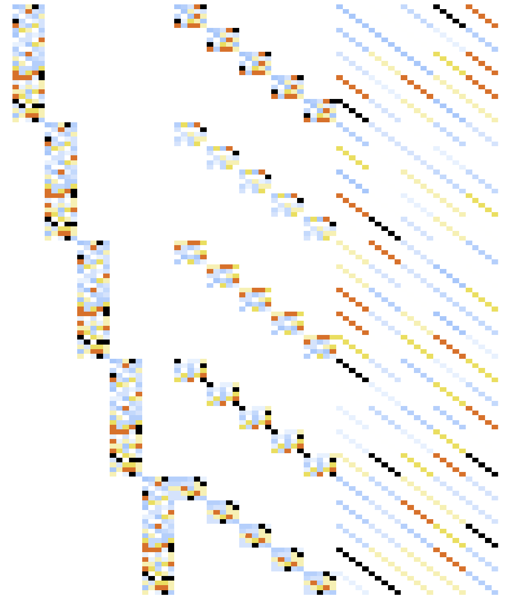
Data layout of the baseline system
We assume for subspaces \(A' \leq A\) and \(B' \leq B\) of dimension \(a'\) and \(b'\), respectively that
Costs:
Total: \(O((a'b'c)(a'r+b's)^2 + (b'cr^2 + a'cs^2) + (b'cu(r+s) + a'cv(r+s))) \)
Full verification omitted - randomized check gives expoentially low probability of error, but complexity to be analyzed.
Restricted system
Compute left inverses
Extend restricted solution
Total: \(O((a'b'c)(a'r+b's)^2 + (b'cr^2 + a'cs^2) + (b'cu(r+s) + a'cv(r+s))) \)
An example fast regime: when \( a,b,c,r,s \) are all \(O(n)\), meaning \(a',b'\) are \(O(1)\)
Total: \(O((c)(r+s)^2 + (cr^2 + cs^2) + (cu(r+s) + cv(r+s))) \)
Plug in \(n\) for \(a,b,c,r,s\), we get the total as \(O((n)(n+n)^2 + (nn^2 + nn^2) + (nn(n+n) + nn(n+n))) = O(n^3) \)
Compared to solving a system of \(n^3\) equations with \(n^2\) variables: \(O(n^3(n^2)^2) = O(n^7)\)
If we add code to check solutions deterministically, need to multiply a \(n^2 \times n\) matrix by a \(n \times n\) matrix, which is \(O(n^4)\) naively. But randomly checking a few linear combinations gives expoentially good probability of correct verification
Derivation Equation
Let \(A,B,C,R,S, T \) be vector spaces with dimensions \(a,b,c,r,s,t\)
Given
\(\rho : \textcolor{blue}{R} \times B \times C \rightarrowtail K \),
\( \sigma : A \times \textcolor{green}{S} \times C \rightarrowtail K \),
\( \tau : A \times B \times \textcolor{orange}{T} \rightarrowtail K \)
Find
\( x : A \rightarrow \textcolor{blue}{R}, y : B \rightarrow \textcolor{green}{S}, z : C \rightarrow \textcolor{orange}{T} \) such that
\[ \rho(x(-),-,-) + \sigma(-,y(-),-) = \tau(-,-,z(-)) \]
as trilinear maps \(A \times B \times C \rightarrowtail K\)
Objective: Given data for this problem in coordinates, report the system is inconsistent or find a non-zero solution faster than solving a linear system with \(abc\) constraints and \(ar + bs + ct \) variables.
Convention:
Observation: (very similar to Simultaneous Sylvester)
Same as before, \(\rho: R \times B \times C \rightarrowtail K \) can be thought of as an element \( \text{Hom}(R, B \otimes C) \). Similar for \(\sigma \in \text{Hom}(S, A \otimes C)\) and \(\tau \in \text{Hom}(T, A \otimes B)\)
Let us assume \(\rho,\sigma,\tau\) are all injective maps. Same as the Sylvester case, this can be done by preprocessing.
Terminology: We call the system \((\tilde{\rho}, \tilde{\sigma}, \tilde{\tau})\) restricted, and to differentiate, and call the full system \((\rho,\sigma,\tau)\) global.
Suppose we have subspaces \(A' \leq A, B' \leq B, C' \leq C\) such that
We solve the restricted system for \(\tilde{x}: A' \rightarrow R, \tilde{y}: B' \rightarrow S, \tilde{z}: C' \rightarrow T \). This means we want the equation \(\tilde{\rho}(\tilde{x}) + \tilde{\sigma}(\tilde{y}) = \tilde{\tau}(\tilde{z})\) to be satisfied.
Choose complements \(A = A' \oplus U\), \(B = B' \oplus V\), and \(C = C' \oplus W\)
Restricting to \(U \leq A\), \(B' \leq B\), and \(C' \leq C\) for \(\rho,\sigma,\tau \) results in the equation \( \rho|_{R \times B'\times C'}(x_U) + \sigma|_{U \times S \times C'}(\tilde{y}) = \tau|_{U \times B' \times T}(\tilde{z}) \)
Notice the first term is the only one with unknowns (being \(x_U\)) and \(\rho|_{R \times B \times C'}: R \times B' \times C' \rightarrowtail K \cong \text{Hom}(R, B'\otimes C')\) is left invertible
Hence solving for \(x_U\) does not require solving a linear system, but rather, just an application of the left inverse, \(\rho|_{R \times B' \times C'}^{\#}\), to all terms.
Projecting to \(A' \leq A\), \(V \leq B\), \(C' \leq C\) finds us \(y_V\) without solving a system of equations.
And projecting to \(A' \leq A, B' \leq B, W \leq C\) finds us \(z_W\) without solving a system of equations.
We call \(x \coloneqq \tilde{x} \oplus x_U\), \(y \coloneqq \tilde{y} \oplus y_V\), and \(z \coloneqq \tilde{z} \oplus z_W\) an extended candidate solution
So the final step is verifying that the unchecked parts of our global system are satisfied by the extended candidate solution. Explicitly, we verify on the spaces
Notation: Denote the direct sum of these spaces as \(M\)
What if the restricted system \( (\tilde{\rho},\tilde{\sigma},\tilde{\tau}) \) is already inconsistent?
Then we can immediately report the overall system \( (\rho,\sigma,\tau) \) is inconsistent, as any solution of the overall system must also solve the restricted one.
On the other hand, if the restricted system has a solution, it will not be unique. So we handle it similarly to the homogeneous case of the Sylvester system.
We will need to search for a solution in the solution space of \( (\tilde{\rho}, \tilde{\sigma}, \tilde{\tau}) \) that extends to a global solution of \((\rho,\sigma,\tau)\)
The correctness of this method is because the the global system \((\rho,\sigma,\tau)\) has a superset of the constraints of the restricted system \( (\tilde{\rho}, \tilde{\sigma}, \tilde{\tau}) \)
Same as the Sylvester case, let \(x \coloneqq \tilde{x} \oplus x_U\), \(y \coloneqq \tilde{y} \oplus y_V\), and \(z \coloneqq \tilde{z} \oplus z_W\) be the extended candidate solution
Define the residual \(\mathcal{E}_{\tilde{x}, \tilde{y}, \tilde{z}}: M \rightarrowtail K\) as \( \mathcal{E}_{\tilde{x},\tilde{y}, \tilde{z}} = \rho(x) + \sigma(y) - \tau(z)\), with the domain restricted to \(M\)
We want a restricted system solution \((\tilde{x}, \tilde{y},\tilde{z})\) whose residual \(\mathcal{E}_{\tilde{x},\tilde{y},\tilde{z}}\) is zero.
Suppose the solution space of \((\tilde{\rho},\tilde{\sigma},\tilde{\tau})\) is given by a vector subspace of dimension \(d\) with \((\tilde{x}_i, \tilde{y}_i, \tilde{z}_i)_{i=1}^{d}\) as a basis.
To set this up, we need the notation: \( \mathcal{E}_i \coloneqq \mathcal{E}_{\tilde{x}_i,\tilde{y}_i, \tilde{z}_i} \)
Now our problem is to solve for \(\lambda_i\) such that \(\sum_i \lambda_i \mathcal{E}_{i} = 0 \). This is a linear algebra problem with \(M\) constraints and \(d\) variables. The core idea of this approach to solving the Derivation System is that d will frequently be small relative to the initial number of variables \(ar + bs + ct\)
A successful solve means the extended candidate solution must be global solution to the system \((\rho,\sigma,\tau)\).
For \(\lambda \coloneqq (\lambda_i)_{i=1}^{d}\), define \((\tilde{x}(\lambda), \tilde{y}(\lambda), \tilde{z}(\lambda))\) as \((\sum_i \lambda_i \tilde{x}_i, \sum_i \lambda_i \tilde{y}_i, \sum_i \lambda_i \tilde{z}_i )\). Similarly, define \(x(\lambda), y(\lambda), z(\lambda)\) as the corresponding extended candidate solution
We solve for a \(\lambda\) giving a valid global solution.
Solving the Derivation System in coordinates
Let \([\rho] \in K^{bc \times r}, [\sigma] \in K^{ac \times s}, [\tau]\in K^{ab \times t}\) be the input to the Derivation system with the appropriate permutations applied to them.
The baseline \(abc\) rows by \(ar + bs + ct\) variables system is laid out by \( (I_a \otimes [\rho]) \text{Vec}(X) + \Pi_{a,b}(I_b \otimes [\sigma]) \text{Vec}(Y) = ([\tau] \otimes I_c) \text{Vec}(Z)\), where \( \Pi_{a,b}\) permutes an element in \(K^{bac \times bs}\) to \(K^{abc \times bs}\).
Arithmetic complexity: \(O((abc)(ar+bs + ct)^2)\) when \(abc \geq ar + bs + ct\)
Data layout
We assume for random subspaces \(A' \leq A\), \(B' \leq B\) and \(C' \leq C\) of dimension \(a', b', c'\) respectively that
Costs:
Continue to account for cost
Full verification omitted - randomized check gives expoentially low probability of error, but complexity to be analyzed.
Restricted system
Compute left inverses
Extend restricted solution
Total: \(O((a'b'c'(a'r+b's+c't)^2) + (b'c'r^2 + a'c's^2 + a'b't^2) + (b'c'u+a'c'v+a'b'w)(r+s+t)) \)
An example fast regime: when \( a,b,c,r,s,t \) are all \(O(n)\), and \(a',b',c'\) are \(O(\sqrt{n})\)
Plug in \(n\) for \(a,b,c,r,s,t\), and \(\sqrt{n}\) for \(a',b',c'\), and we get the total as \(O((\sqrt{n}\sqrt{n}\sqrt{n}(\sqrt{n}n+\sqrt{n}n+\sqrt{n}n)^2) + (\sqrt{n}\sqrt{n}n^2 + \sqrt{n}\sqrt{n}n^2 + \sqrt{n}\sqrt{n}n^2) + (\sqrt{n}\sqrt{n}n+\sqrt{n}\sqrt{n}n+\sqrt{n}\sqrt{n}n)(n+n+n)) \)
Compared to solving a system of \(n^3\) equations with \(n^2\) variables: \(O(n^3(n^2)^2) = O(n^7)\)
Total: \(O((a'b'c'(a'r+b's+c't)^2) + (b'c'r^2 + a'c's^2 + a'b't^2) + (b'c'u+a'c'v+a'b'w)(r+s+t)) \)
Simplifies to \(O(n^{1.5}(n^{1.5})^2 + (n^3 + n^3 + n^3) + (n^2 + n^2 + n^2)(n+n+n)\) = \(O(n^{4.5}) \)
By Chris Liu


