Efficient Estimation of Word Representations in Vector Space
Mikolov et al
Motivation
- Difficult to learn relationships between words
- Current methods require significant computation
Objective
- Learn high-quality word vectors
- Billions of words in dataset
- Millions of word in vocabulary
- Hundreds of features in vectors
- Recognize syntactic and semantic word similarities
- Preserve linear regularities among words
Basic Results
- Two novel architectures
- Lower computation
- Improved accuracy
- State of the art performance
- New test to measure syntactic and semantic similarity
Background
N-gram
Examples:
- "The quick brown fox jumped over the lazy dog."
- 1-gram: "the," "quick," "brown,"...
- 2-gram: "the quick," "quick brown," "brown fox,"...
- 3-gram: "the quick brown," "quick brown fox,"...
- Can be sequences of characters too
N-gram model
- Statistical
- Given a sequence, can one predict the next gram?
- Goal: learn important combinations of words
N-gram model
Advantages:
- Simple
- Robust
- Simple models + huge datasets → good performance
N-gram model
Disadvantages
- Limited data
- Millions of words for speech recognition
- Advances in ML → better, more complex models
- Neural networks outperform N-gram
Word Vectors
- Represent words as continuous feature vectors
- Vectors are continuous random variables in \(\mathbb{R}^n\)
- Relationship between words (cosine distance)
Architecture Comparison
- (Feedforward) Neural Net Language Model (NNLM)
- Recurrent Neural Net Language Model (RNNLM)
- New Models:
- Continuous Bag-of-Words Model (CBOW)
- Continuous Skip-gram Model
Training Complexity
- \(E:\) number of epochs, \(\approx3-50\)
- \(T:\) number of words in training set, \(\approx 10^9\)
- \(Q:\) complexity of model architecture
O=E\times T\times Q
Previous Models
Neural Network
Language Model (NNLM)
- Curse of dimensionality
- Solution:
- Create word vectors in \(R^m\) \( (m<<|V|)\)
- Jointly learn vectors and statistical language model
- Generalizable
Neural Network
Language Model (NNLM)
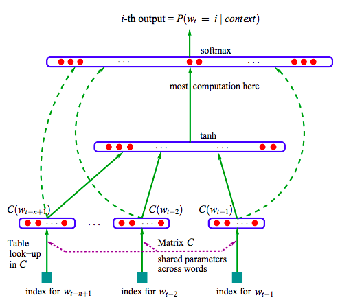
NNLM Complexity
- \(V\): vocabulary size, \(\approx 10^6\)
- \(N\): previous words, \(\approx 10\)
- \(P=ND\): dimension of projection layer, \(\approx 500-2000\)
- \(H\): hidden layer size, \(\approx 500-1000\)
Q=ND+NDH+HV
NNLM: Advantages
- Generalizes
- "The dog was running in the room."
- \(dog\approx cat, walking\approx running, room\approx bedroom\)
- "The cat was walking in the bedroom"
- Complex so can be precise
NNLM: Disadvantages
- Complex
NNLM: Modification
- First learn word vectors
- Neural network, single hidden layer
- Then use vectors to train NNLM
- This paper: learning word vectors better
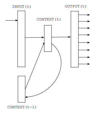
Recurrent NNLM:
- Connects to itself, using time-delayed connection
- No projection layer
- Natural for patterns involving sequences
RNNLM
RNNLM Complexity
Q=DH+HV
RNNLM: Advantages
- No need to specify context length (\( N\))
- Short term memory
- Efficient representation for complex patterns (vs. NN)
RNNLM: Disadvantages
- Complex, but less than NNLM
- Parallelizes poorly
New Models
New Models
- Remove hidden layer to reduce complexity
- Less precision, higher efficiency
Continuous Bag-of-Words
- Similar to NNLM with no hidden layer
- All words share projection layer
- Order of words does not influence projection
- Includes words from future
- Future and history words as input
- Goal: Correctly classify missing middle word
CBOW Architecture
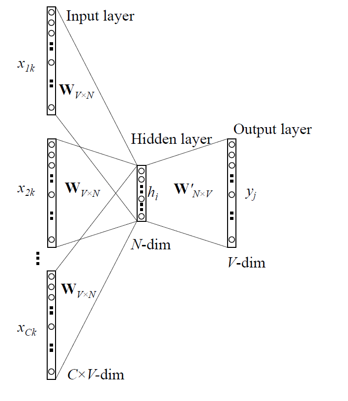
CBOW Complexity
Q=ND+D\log(V)
Continuous Skip-gram
- Inverse of CBOW
- Current word is input
- Surrounding words are output
- Larger range improves quality, increases complexity
- Distant words less related, sampled less
Skip-gram Architecture
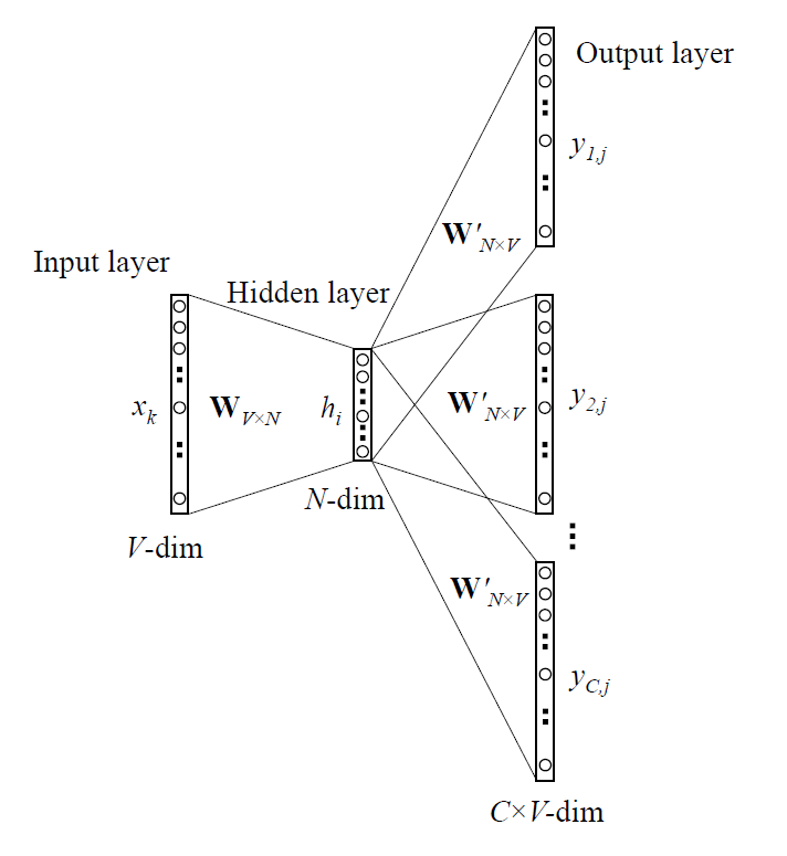
Skip-gram complexity
- \(C\): Maximum distance of the words, \(\approx 10\)
- Randomly select \(R\) in range \([1,C]\)
- Use \(R\) from history and \(R\) from future
- Current word input, \(2R\) words output
Q=CD+CD\log(V)
Training
Learning Model: CBOW
- Learning Type: Supervised
- Input: Surrounding words
- Output: Correctly identified missing word
- Hypothesis Set: Modified feedforward NNLM
- Learning Algorithm: Stochastic gradient descent, back propagation
- \(f\): ideal function picking missing current word from surrounding words
Learning Model: Skip-gram
- Learning Type: Supervised
- Input: Current word
- Output: Correctly identified surrounding words
- Hypothesis Set: Modified feedforward NNLM
- Learning Algorithm: Stochastic gradient descent, back propagation
- \(f\): ideal function picking surrounding words from current word
Training Type
- Small data: Gradient descent, linearly decreasing learning rate, single CPU
- Large data: Mini-batch asynchronous gradient descent, adaptive learning rate Adagrad, DistBelief
- \(\approx 100\) model replicas, each with many CPUs on different machines
Function Maximization
and Error
- CBOW maximizes: \[p(w_O|w_{I,1},\dots,w_{I,N})\]
- Skip-gram maximizes: \[p(w_{O,1},\dots,w_{O,C}|w_I)\]
- Error function for both: log-loss
Evaluation
Typical Approach
- Pick a word, and list most similar words
- France:
| spain | 0.678 |
| belgium | 0.666 |
| netherlands | 0.652 |
| italy | 0.633 |
| switzerland | 0.622 |
| luxembourg | 0.610 |
New Approach
- More complex similarity task
- "What is the word that is similar to small in the same sense as biggest is similar to big?"
- Word vectors (perhaps surprisingly) work like vectors
vector(X)=vector(``biggest")-vector(``big")+vector(``small")
- Search vectors for word closest to X (cosine distance)
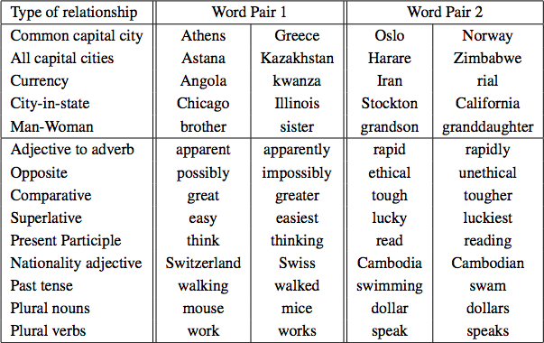
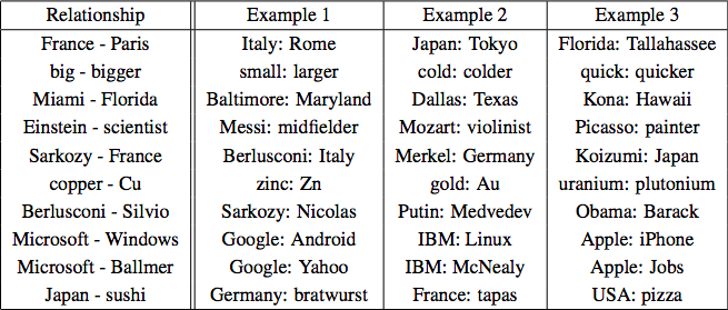
Test
- Novel Test
- Five types of semantic questions
- Nine types of syntactic questions
- Question generation:
- Manually create list of similar word pairs
- Connect two word pairs to form question
- Correct answer: only if closest word is exact same
- Synonyms are mistakes
Five semantic and nine syntactic questions in the Semantic-Syntactic Word Relationship test set
Results
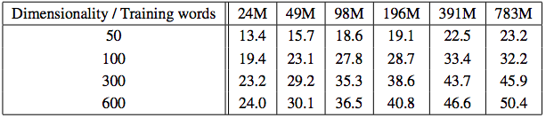
Dimensions vs. Data
- Must increase in size together
- Currently popular to have big data and small vectors
- CBOW:
Epochs vs. Data
- 3 epochs \(\approx\) 1 epoch, double the data
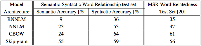
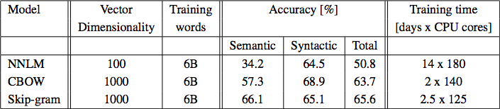
Results for the Four Models
- Vector dimension: 640
- Dataset: LDC, 320M words, 82K vocab
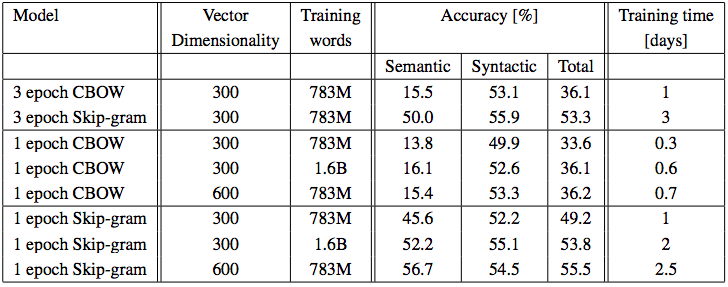
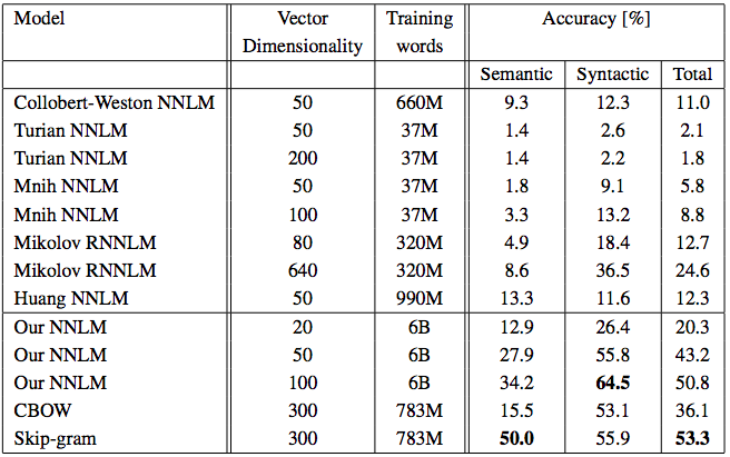
Results vs. Other Models
- CBOW and Skip-gram trained on Google News subset
Large Scale Parallel Training
- DistBelief
- Dataset: Google News, 6B words
- Mini-batch asynchronous gradient descent
- Adagrad adaptive learning rate
Microsoft Sentence Completion Challenge
- 1040 sentences, one word missing in each
- Five reasonable choices
- Use Skip-gram, pick word from options and predict surrounding words in sentence
"That is his
[ generous | mother’s | successful | favorite | main ]
fault , but on the whole he’s a good worker."
MSCC Results

Additive Results:
- Skip gram, 783M words, 300 dimensionality
Conclusion and Future
- Can build good word vectors with simple models
- Not good at words with multiple meanings
- Now:
- Skip-gram and CBOW are common and faster
- 100B words, 300 dimensions, 3 million vocab
- Can handle short phrases: new_york
- Can be used for clustering:
- acceptance, argue, argues, arguing, argument, arguments, belief, believe, challenge, claim
Analysis
- Results for both CBOW and Skip-gram
- EX: MSCC seems perfect for CBOW
- Maybe they don't have a good answer for when the word isn't in the options
- Could have combined them for that?
- EX: MSCC seems perfect for CBOW
- Unclear on many specifics
- EX: Error function, hyperparameter setting
NNML
By Connor Chapin
NNML
Presentation on "Efficient Estimation of Word Representations in Vector Space"