


Content ITV PRO
This is Itvedant Content department
Reduce Dimensions Using PCA for Better Insights
Business Scenario
Welcome!
Today is your ninth day as a Junior Data Scientist at MediCare Analytics.
Our company has recently partnered with a network of hospitals and healthcare research centers to improve the understanding of heart disease risk factors using patient health records.
The client has shared a medical dataset containing patient information such as age, cholesterol levels, blood pressure, heart rate, chest pain type, ECG results, and other clinical measurements.
Although the dataset contains valuable information, it contains multiple health indicators that make visualization and interpretation difficult. The healthcare team wants to simplify the dataset while preserving the most important information so that researchers can better understand patient health patterns.
Before building advanced predictive models, your manager wants you to understand how Dimensionality Reduction can simplify complex datasets and improve data visualization.
As part of this project, you will:
Pre-Lab Preparation
Topic : Unsupervised Learning
1) PCA
git pull origin branchNameGit Pull
Task 1: Understanding Dimensionality Reduction
Before applying PCA, it is important to understand why dimensionality reduction is needed in machine learning projects.
What is Dimensionality Reduction?
Dimensionality Reduction is the process of reducing the number of features in a dataset while preserving as much useful information as possible.
Datasets with many variables are often difficult to analyze and visualize. Dimensionality reduction helps simplify the dataset and improves computational efficiency.
Benefits of Dimensionality Reduction
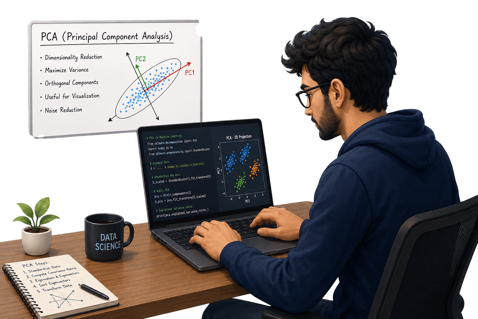
What is PCA?
Principal Component Analysis (PCA) is an unsupervised machine learning technique used for dimensionality reduction.
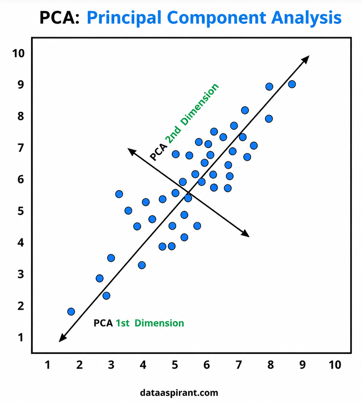
PCA transforms the original features into a smaller set of new variables called Principal Components. These components capture the maximum variance present in the dataset.
The first principal component captures the highest variance, followed by the second principal component, and so on.
Advantages of PCA
Task 2: Applying PCA for Better Insights
Now that you understand dimensionality reduction, the healthcare analytics team wants you to apply PCA on patient health records.
The objective is to:
Standardize the dataset.
Apply PCA.
Analyze explained variance.
Reduce the dataset into principal components.
Visualize patient distributions.
While performing PCA, think about:
How much variance is explained by each component?
How many principal components should be selected?
Open a new file in Google Colab and import libraries
1
import numpy as np
import pandas as pd
import matplotlib.pyplot as plt
import seaborn as sns

import warnings
warnings.filterwarnings('ignore')
Load and explore dataset
2
Click to download Dataset : heart.csv
df = pd.read_csv("heart.csv")

df.head()
Explore Dataset
3
df.shape
df.info()
df.describe()
Separate Input and Target Variables
4
X = df.drop("target", axis=1)

Y = df["target"]
Split Dataset
5
from sklearn.model_selection import train_test_split

X_train, X_test, Y_train, Y_test = train_test_split(
    X,
    Y,
    test_size=0.3, random_state=1)
Standardize the Dataset
6
from sklearn.preprocessing import StandardScaler

ss = StandardScaler()

X_train = ss.fit_transform(X_train)

X_test = ss.transform(X_test)
Import PCA
7
from sklearn.decomposition import PCAApply PCA
8
pc1 = PCA(
    n_components=None,
    random_state=1
)

X_train1 = pc1.fit_transform(X_train)

X_test1 = pc1.transform(X_test)
Analyze Explained Variance
9
pc1.explained_variance_ratio_Calculate Cumulative Variance
10
np.cumsum(pc1.explained_variance_ratio_)Select Optimal Principal Components
11
pc2 = PCA(
    n_components=6,
    random_state=1
)

X_train1 = pc2.fit_transform(X_train)

X_test1 = pc2.transform(X_test)
Build Logistic Regression Model
12
from sklearn.linear_model import LogisticRegression
lr = LogisticRegression()
lr.fit(X_train1, Y_train)
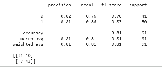
Y_pred = lr.predict(X_test1)Evaluate Model
13
from sklearn.metrics import classification_report
from sklearn.metrics import confusion_matrix

print(classification_report(Y_test, Y_pred))

print(confusion_matrix(Y_test, Y_pred))
Reduce Data to Two Principal Components
14
pca_vis = PCA(n_components=2)
X_pca = pca_vis.fit_transform(
StandardScaler().fit_transform(X)
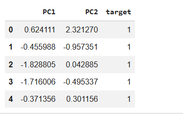
)Create PCA DataFrame
15
pca_df = pd.DataFrame(
data=X_pca,
columns=["PC1", "PC2"]
)
pca_df["target"] = Y
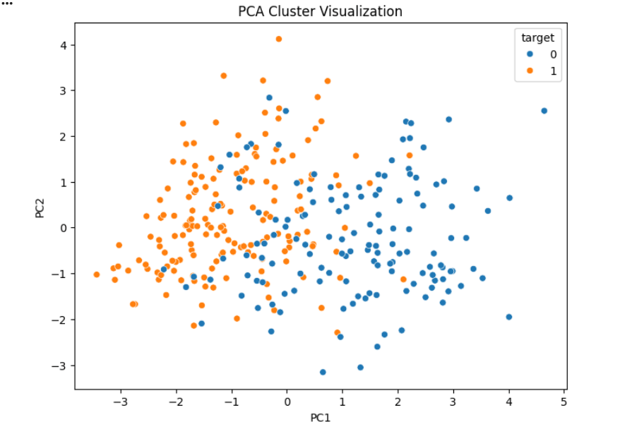
pca_df.head()Visualize Clusters
16
plt.figure(figsize=(8,6))

sns.scatterplot(
    x="PC1",
    y="PC2",
    hue="target",
    data=pca_df
)

plt.title("PCA Cluster Visualization")

plt.show()
Great job!
You have successfully completed lab 15: Reduce Dimensions Using PCA for Better Insights.
In this lab, you have: Understood Dimensionality Reduction, Learned Principal Component Analysis (PCA), Applied PCA on the Heart Disease dataset, Analyzed explained variance, Reduced multiple features into principal components, Evaluated model performance using PCA-transformed data, and Visualized patient clusters using PCA.
You are now ready to move to the next stage of machine learning. In the next lab, we will learn how to Build an ML Web App Using Streamlit and deploy machine learning models through an interactive web interface.
Checkpoint
Git Push
git push origin branchNameNext-Lab Preparation
Topic : Model Deployment Basics
1) Introduction to Streamlit for ML Model Deployment
2) Web Application for ML Predictions
By Content ITV


