
\Delta r
r_\psi(s, a) - r_\psi(s, b)
P(a>b|s)
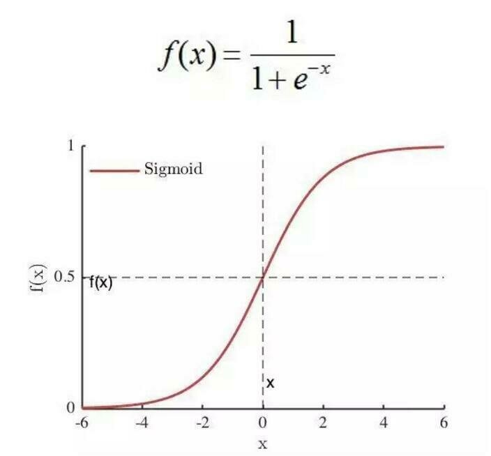
\sigma(x) = \frac{1}{1 + e^{-x}}
x
y
изображение
робота
Оптимальное действие:
\rightarrow
тут обучили награду
тут будут проблемы


Случай известной динамики среды
Планирование с и без обратной связи
What if the environment's model
is given?
Reminder:
p(\tau) = p(s_0)\prod_{t=0}^T \pi(a_t|s_t) p(s_{t+1}|s_t, a_t)
p(s_{t+1}|s_t, a_t)

Previously:
- observed only samples from the environment
- not able to start from an arbitrary state
Now the environment's model is fully accessible:
- can plan in our mind without interaction
- we assume rewards are known too!
or \(s_{t+1} = f(s_t, a_t)\)
Interaction vs. Planning
In deterministic environments
Model-free RL (interaction):


a_t
s_{t+1}, r_t
agent
environment
\pi(a|s)
Interaction vs. Planning
In deterministic environments
Model-based RL (open-loop planning):
agent
environment

a_t, r_t, s_{t+1}, a_{t+1}, r_{t+1}, s_{t+2}, \dots
s.t. \;\; f(s, a) = s'
a_t, a_{t+1}, a_{t+2}, \dots
optimal plan
a_t, a_{t+1}, a_{t+2}, \dots
r_t, s_{t+1}, r_{t+1}, s_{t+2}, r_{t+2}, \dots
Planning in stochastic environments
Plan:


p(G) = 0.1
p(G) = 0.9
Reality:

Closed-loop planning (Model Predictive Control - MPC):
agent
environment
a_t, r_t, s_{t+1}, a_{t+1}, r_{t+1}, s_{t+2}, \dots
s.t. \;\; f(s, a) = s'
a_t, a_{t+1}, a_{t+2}, \dots
optimal plan
a_t
r_t, s_{t+1}
Planning in stochastic environments
Apply only first action!
Discard all other actions!
REPLAN AT NEW STATE!!
How to plan?
Continuous actions:
- Linear Quadratic Regulator (LQR)
- iterative LQR (iLQR)
- Differential Dynamic Programming (DDP)
- ....
Discrete actions:
- Monte-Carlo Tree Search
- ....
- ....


Планирование как поиск по дереву
Tree Search
Deterministic dynamics case
s_0
a_{01}
a_{00}
s_{10}
s_{11}
s_{20}
s_{21}
s_{22}
s_{23}
a_{11}
a_{10}
a_{13}
a_{12}
V(s) = r(s)
V(s) = \max_a V(f(s, a))
r=1
r=0
r=2
r=-1
1
0
2
-1
1
\;\;\;\;\;2
V(s) = \max_a[r(s, a) + \mathbb{E}_{p(s'|s, a)} V(s')] \;\rightarrow\; V(s) = \max_a[r(s, a) + V(s')]
reminder:
-1
Q(s, a) = V(s')
apply \(s' = f(s, a)\) to follow the tree
assume only terminal rewards!
a^* = \arg\max_a Q(s, a)
Tree Search
Deterministic dynamics case
- Full search is exponentially hard!
- We are not required to track states: the sequence of actions contains all the required informations
Tree Search
Stochastic dynamics case
s_0
a_{01}
a_{00}
s_{10}
s_{13}
a_{11}
a_{10}
V(s) = r(s)
V(s) = \max_a Q(s, a)
apply \(s' \sim p(s'|s, a)\) to follow the tree
assume only terminal rewards!
a^* = \arg\max_a Q(s, a)
s_{11}
s_{12}
a_{11}
a_{10}
a_{11}
a_{10}
a_{11}
a_{10}
s
s
s
s
s
s
s
s
s
s
s
s
s
s
s
s
Q(s, a) = \sum_{s'} \hat{p}(s'|s,a)V(s')
Q(s, a) = \sum_{s'} \hat{p}(s'|s,a)V(s')
p(s'|s, a) \approx \hat{p}(s'|s, a) = \frac{n(s')}{n^{parent}(s')}
Now we need an infinite amount of runs through the tree!
Tree Search
Stochastic dynamics case
- The problem is even harder!
If the dynamics noise is small, forget about stochasticity and use the approach for deterministic dynamics.
The actions will be suboptimal.
But who cares...
Монте-Карло поиск по дереву
Monte-Carlo Tree Search (MCTS)
Monte-Carlo Tree Search: v0.5
also known as Pure Monte-Carlo Game Search
R \sim p(R|s)

Simulate with some policy \(\pi_O\) and calculate reward-to-go
s_0
a_{01}
a_{00}
s_{10}
s_{11}
s_{20}
s_{21}
s_{22}
s_{23}
a_{11}
a_{10}
a_{13}
a_{12}
V(s) = \max_a V(f(s, a))
Q(s, a) = V(s')
a^* = \arg\max_a Q(s, a)
V^{\pi_O}(s) = \mathbb{E}_{p(R|s)} R
We need an infinite amount of runs to converge!
Monte-Carlo Tree Search: v0.5
also known as Pure Monte-Carlo Game Search
- Not so hard as full search, but still!
- Will give a plan which is better than following \(\pi_O\), but is suboptimal!
- The better the plan - the harder the problem!
Is it necessary to explore all the actions with the same frequency?
Maybe we'd better explore actions with a higher estimate of \(Q(s, a)\) ?
At an earlier stage, we also should have some exploration bonus for the least explored actions!
Upper Confidence Bound for Trees
UCT
Basic Upper Confidence Bound for Bandits:
Th.: Given some assumptions the following is true:
\mathbb{P}\Big(Q(a) - \hat{Q}(a) \ge \sqrt{\frac{2}{n(a)}\log\big(\frac{1}{\delta}\big)} \Big) \le \delta
Upper Confidence Bound bonus for MCTS:
We should choose actions that maximize the following value:
W(s, a) = \hat{Q}(s, a) + c\sqrt{\frac{\log n^{parent}(s)}{n(a)}}
s_0
a_{01}
a_{00}
Monte-Carlo Tree Search: v1.0
R \sim p(R|s)
Simulate with some policy \(\pi_O\) and calculate reward-to-go
a_{01}
a_{00}
s_{10}: (0, 0)
s_{11} : (0, 0)
s_{20}: (0, 0)
s_{21}: (0, 0)
s_{22}: (0, 0)
a_{11}
a_{10}
a_{13}
a_{12}
V(s) = \frac{\Sigma}{n(s)}
\pi_I(s) = \arg\max_a W(s, a)
W(s, a) = V(s') + c\sqrt{\frac{\log n(s)}{n(a)}}
For each state we store a tuple:
\( \big(\Sigma, n(s) \big) \)
\(\Sigma\) - cummulative reward
\(n(s)\) - counter of visits
Stages:
- Forward
- Expand
- Rollout
- Backward
W = \infty
W = \infty
s_{10}: (1, 1)
s_{11} : (0, 1)
W = 1 + c
W = c \sqrt{\ln2}
W = 1 + c\sqrt{\ln2}
W = 1 + \sqrt{\ln2}
W = \infty
s_{20}: (1, 1)
s_{10}: (2, 2)
s_0
W = 1 + c\sqrt{\frac{\ln3}{2}}
W = c \sqrt{\ln3}
W = \infty
W = \infty
W = \infty
s_{22}: (-1, 1)
s_{11} : (-1, 2)
W = -\frac{1}{2} + c \sqrt{\frac{\ln4}{2}}
W = 1 + c \sqrt{\frac{\ln4}{2}}
s_{21}: (-2, 1)
s_{10}: (0, 3)
and again, and again....
Monte-Carlo Tree Search
Python pseudo-code
def mcts(root, n_iter, c):
    for n in range(n_iter):
    	leaf = forward(root, c)
        reward_to_go = rollout(leaf)
        backpropagate(leaf, reward_to_go)
    return best_action(root, c=0)
def forward(node, c):
    while is_all_actions_visited(node):
        a = best_action(node, c)
        node = dynamics(node, a)
    if is_terminal(node):
        return node
    a = best_action(node, c)
    child = dynamics(node, a)
    add_child(node, child)
    return child
def rollout(node):
while not is_terminal(node):
a = rollout_policy(node)
node = dynamics(node, a)
return reward(node)def backpropagate(node, reward):
if is_root(node):
return None
node.n_visits += 1
node.cumulative_reward += reward
node = parent(node)
return backpropagate(node, reward)Моделирование оппонента
в настольных играх
Minimax MCTS

agent

environment
The environment's dynamics is unknown!
environment
The environment's dynamics is now known!

agent
maximizing return
minimizing return
Minimax MCTS
There are just a few differences compared to the MCTS v1.0 algorithm:
- Now you should track which player's move is now
- \(o = 1\;\; \texttt{if player's 1 move, else}\;\; -1 \)
- During forward pass, best actions now should maximize:
\(W(s, a) = oV(s') + c\sqrt{\frac{\log n(s)}{n(a)}}\)
- The best action, computed by MCTS is now:
\(a^* = \arg\max_a oQ(s, a) \)
- Other stages are not changed at all!
Улучшение стратегии
с помощью
Монте-Карло поиска по дереву
Policy Iteration guided by MCTS
You may have noted that MCTS looks something like this:
- Estimate value \(V^{\pi_O}\) for the rollout policy \(\pi_O\) using Monte-Carlo samples
- Compute it's improvement as \(\pi_O^{MCTS}(s) \leftarrow MCTS(s, \pi_O)\)
But then we just throw \(\pi_O^{MCTS}\) and \(V^{\pi_O}\) away and recompute them again!
We can use two Neural Networks to simplify and improve computations:
- \(V_\phi\) that will capture state-values and will be used instead of rollout estimates
- \(\pi_\theta\) that will learn from MCTS improvements
MCTS algorithm from AlphaZero
During the forward stage:
- At leaf states \(s_L\), we are not required to make rollouts - we already have its value:
\(V(s_L) = V_\phi(s_L)\)
or we can still do a rollout: \(V(s_L) = \lambda V_\phi(s_L) + (1-\lambda)\hat{V}(s_L)\)
- The exploration bonus is now changed - the policy guides exploration:
\(W(s') = V(s') + c\frac{\pi_\theta(a|s)}{1+ n(s')}\)
There are no infinite bonuses
s
a
s'
Now, the output of MCTS\((s)\) is not the best action for \(s\), but rather a distribution:
\( \pi_\theta^{MCTS}(a|s) \propto n(f(s, a))^{1/\tau}\)
Other stages are not affected.
Assume, we have a rollout policy \(\pi_\theta\) and a corresponding value function \(V_\phi\)
But how to improve parameters \(\theta\)?
And update \(\phi\) for the new policy?
Policy Iteration through a self-play
s_0
Play several games with yourself:

R
Keep the tree through the game!
a_0 \sim \pi_\theta^{MCTS}(s_0)
s_1
a_1 \sim \pi_\theta^{MCTS}(s_1)
. . .
s_T
a_T \sim \pi_\theta^{MCTS}(s_T)
Store the triples: \( (s_t, \pi_\theta^{MCTS}(s_t), R), \;\; \forall t\)
Once in a while, sample batches \( (s, \pi_\theta^{MCTS}, R) \) from the buffer and minimize:
l = (R - V_\phi(s))^2 - ( \pi_\theta^{MCTS} )^T \log \pi_\theta(s) + \kappa ||\theta||^2_2 + \psi ||\phi||^2_2
Better to share parameters of NNs
AlphaZero results


AlphaZero results


AlphaZero results

Случай неизвестной динамики
What if the dynamics is unknown?
\( f(s, a) \) - ????
If we assume dynamics to be unknown but deterministic,
then we can note the following:
- states are fully controlled by applied actions
- during MCTS search the states are not required
in case of known \( V^{\pi_O}(s), \pi_O(s), r(s) \)
(rewards are here for more general environments than board-games)
we can learn it directly from transtions of a real environment
What if the dynamics is unknown?
The easiest motivation ever!
Previously, in AlphaZero we had:
Now the dynamics is not available!
Thus, we will throw all the available variables into a larger NN:
\(s_{root}, a_0, \dots, a_L\)
dynamics
\(s_L\)
get value and policy
\(V_\theta (s_L), \pi_\theta (s_L) = f_\theta(s_L)\)
\(s_{root}, a_0, \dots, a_L\)
get value and policy of future states
\(V_\theta (s_L), \pi_\theta (s_L) = f_\theta(s_L)\)
Architecture of the Neural Network
the estimate of r(s, a)
a_{t+1}
\(g_\theta(z_{t+1}, a_{t+1}) \)
\rho_{t+1}
z_{t+2}
\(f_\theta(z_{t+2}) \)
V_{t+2}
\pi_{t+2}
. . .
. . .
encoder
z_t
a_t
\(g_\theta(z_t, a_t) \)
\rho_t
z_{t+1}
\(f_\theta(z_{t+1}) \)
V_{t+1}
\pi_{t+1}
s_t
MCTS in MuZero
R \sim p(R|s)
Simulate with some policy \(\pi_O\) and calculate reward-to-go
a_{01}
a_{00}
s_{10}: (0, 0)
s_{11} : (0, 0)
s_{20}: (0, 0)
s_{21}: (0, 0)
s_{22}: (0, 0)
a_{11}
a_{10}
a_{13}
a_{12}
V(s) = \frac{\Sigma}{n(s)}
\pi_I(s) = \arg\max_a W(s, a)
W(s, a) = V(s') + c\sqrt{\frac{\log n(s)}{n(a)}}
For each state we store a tuple:
\( \big(\Sigma, n(s) \big) \)
\(\Sigma\) - cummulative reward
\(n(s)\) - counter of visits
Stages:
- Forward
- Expand
- Rollout
- Backward
W = \infty
W = \infty
s_{10}: (1, 1)
s_{11} : (0, 1)
W = 1 + c
W = c \sqrt{\ln2}
W = 1 + c\sqrt{\ln2}
W = 1 + \sqrt{\ln2}
W = \infty
s_{20}: (1, 1)
s_{10}: (2, 2)
s_0
W = 1 + c\sqrt{\frac{\ln3}{2}}
W = c \sqrt{\ln3}
W = \infty
W = \infty
W = \infty
s_{22}: (-1, 1)
s_{11} : (-1, 2)
W = -\frac{1}{2} + c \sqrt{\frac{\ln4}{2}}
W = 1 + c \sqrt{\frac{\ln4}{2}}
s_{21}: (-2, 1)
s_{10}: (0, 3)
and again, and again....
a_{00}
a_{11}
s_0
s_{21}: (-2, 1)
s_{10}: (0, 3)
MCTS in MuZero
R \sim p(R|s)
Simulate with some policy \(\pi_O\) and calculate reward-to-go
\pi_I(s) = \arg\max_a W(s, a)
W(s, a) = V(s') + c\sqrt{\frac{\log n(s)}{n(a)}}
Stages:
- Forward
- Expand
- Rollout
- Backward
W = 1 + c \sqrt{\frac{\ln4}{2}}
W = \infty
MuZero: article
s_0
Play several games:
a_0 \sim \pi_\theta^{MCTS}(s_0)
s_1
a_1 \sim \pi_\theta^{MCTS}(s_1)
. . .
s_T
a_T \sim \pi_\theta^{MCTS}(s_T)
Store whole games: \( (..., s_t, a_t, \pi_t^{MCTS}, r_t, u_t, s_{t+1}, ...)\)
Randomly pick state \(s_i\) from the buffer with a subsequence of length \(K\)
l = \sum_{k=0}^K (u_{i+k} -v_k)^2 + (r_{i+k} - \rho_k)^2 - ( \pi_{i+k}^{MCTS} )^T \log \pi_k + \kappa ||\theta||^2_2
r_0
r_1
r_T
u_t = \sum_{t'=t}^{T}\gamma^{(t'-t)}r_{t'}
v_k, \pi_k, \rho_k = NN(s_i, a_i, \dots, a_{i+k})
MuZero: results

MuZero: results


WOW
It works!
OpenEdu MB-RL: MCTS, AlphaZero, MuZero
By cydoroga


