


Davide Murari
A PhD student in numerical analysis at the Norwegian University of Science and Technology.
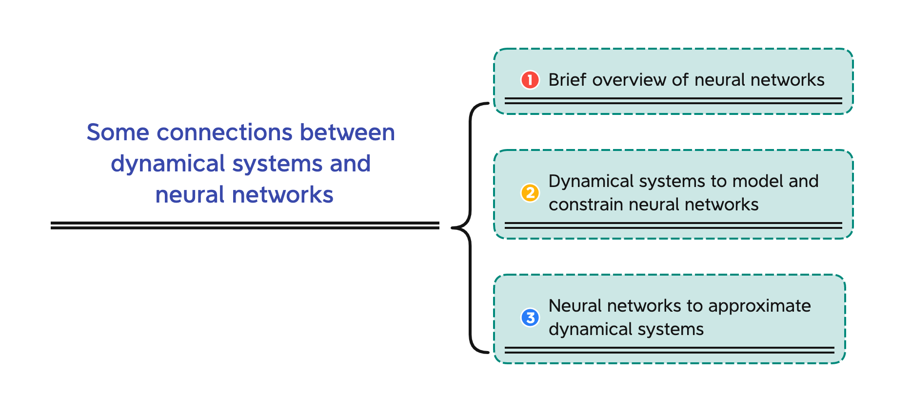
Some connections between dynamical systems and neural networks
Davide Murari
Veronesi Tutti Math Seminar - 06/04/2022
\(\texttt{davide.murari@ntnu.no}\)
What is supervised learning
Consider two sets \(\mathcal{C}\) and \(\mathcal{D}\) and suppose to be interested in a specific (unknown) mapping \(F:\mathcal{C}\rightarrow \mathcal{D}\).
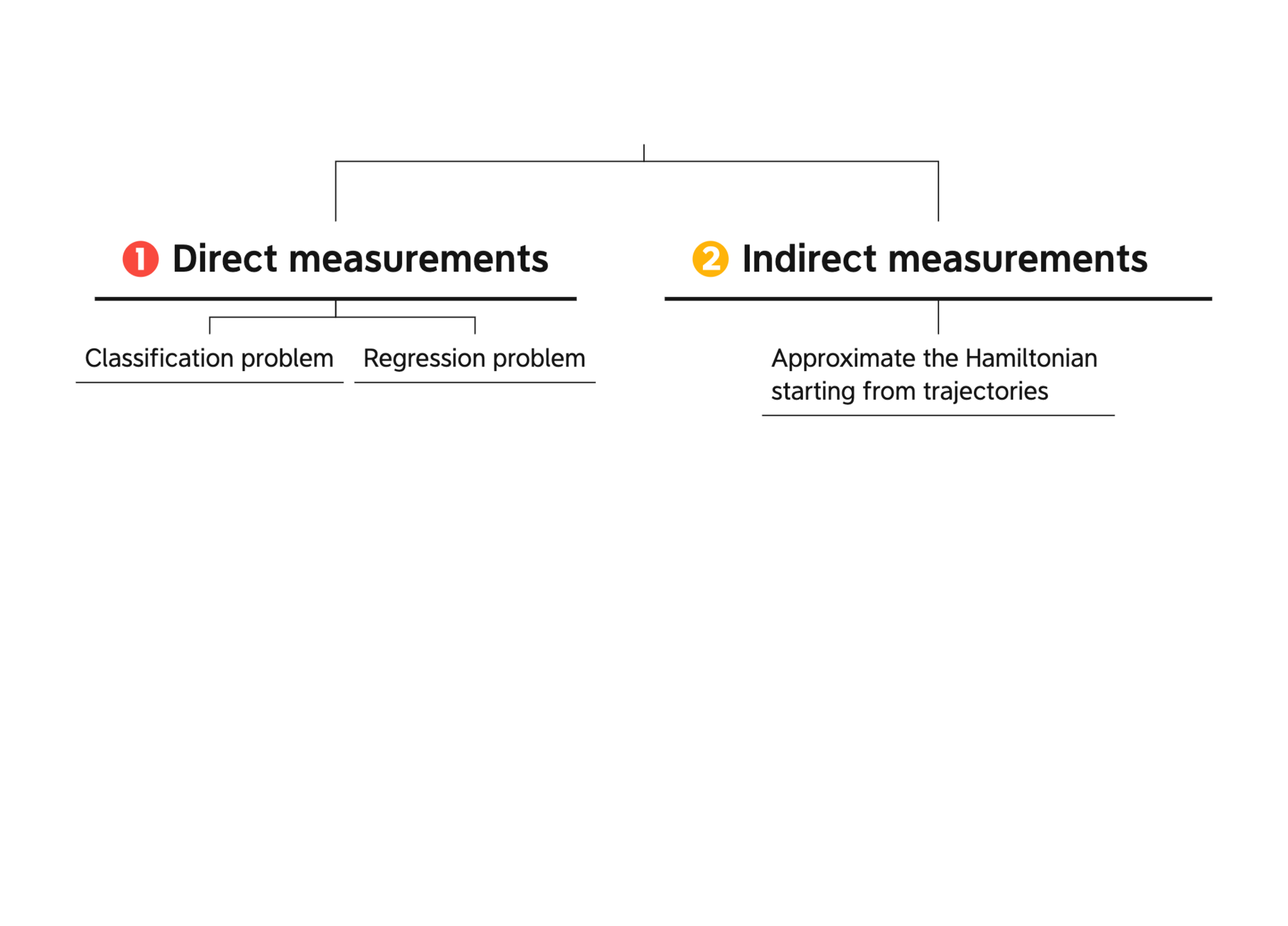
The data we have available can be of two types:
GOAL: Approximate \(F\) on all \(\mathcal{C}\).
Examples of these tasks
What are neural networks
What are neural networks
They are compositions of parametric functions
\( \mathcal{NN}(x) = f_{\theta_k}\circ ... \circ f_{\theta_1}(x)\)
Examples
\(f_{\theta}(x) = x + B\Sigma(Ax+b),\quad \theta = (A,B,b)\)
ResNets
Feed Forward
Networks
\(f_{\theta}(x) = B\Sigma(Ax+b),\quad \theta = (A,B,b)\)
\(\Sigma(z) = [\sigma(z_1),...,\sigma(z_n)],\quad \sigma:\mathbb{R}\rightarrow\mathbb{R}\)
Neural networks motivated by dynamical systems
EXPLICIT
EULER
\( \Phi_{f_i}^{h_i}(x) = x + h_i f_i(x)\)
\( \dot{x}(t) = f(t,x(t),\theta(t)) \)
Time discretization : \(0 = t_1 < ... < t_k <t_{k+1}= T \), \(h_i = t_{i+1}-t_{i}\)
Where \(f_i(x) = f(t_i,x,\theta(t_i))\)
EXAMPLE
\(\dot{x}(t) = \Sigma(A(t)x(t) + b(t))\)
Imposing some structure
1-LIPSCHITZ NETWORKS
HAMILTONIAN NETWORKS
VOLUME PRESERVING, INVERTIBLE
Hamiltonian systems
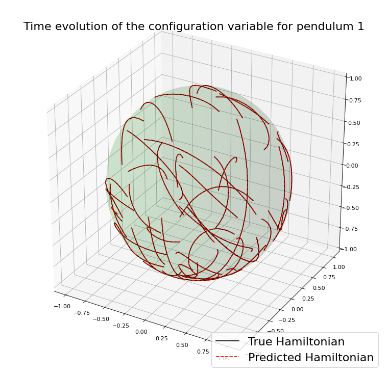
Approximating Hamiltonian systems with neural networks
GOAL: Approximate a Hamiltonian vector field \(X_H\in\mathfrak{X}(\mathbb{R}^{2n})\)
DATA: \(\mathcal{T} = \{(x_i,y_i^1,...,y_i^M)\}_{i=1,...,N}\)
\(y_i^j = \phi_{X_H}^{jh}(x_i) + \delta_i^j \)
KINETIC
ENERGY
POTENTIAL
ENERGY
\(\Theta=(\theta_1,...,\theta_k,A)\)
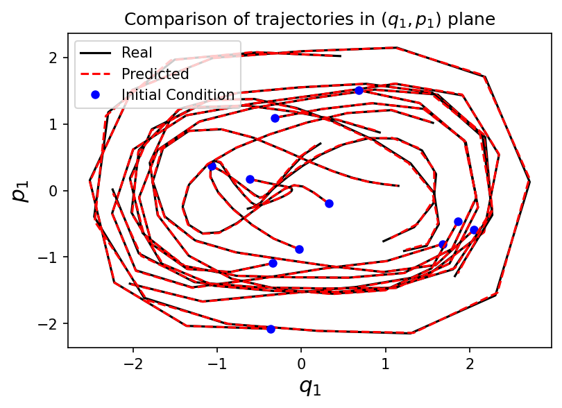
Approximating Hamiltonian systems with neural networks
\( Y_{\Theta}(q,p) = X_{\mathcal{NN}_{\Theta}}(q,p) = \mathbb{J}\nabla \mathcal{NN}_{\Theta}(q,p) \)
\( \Phi^h_{Y_{\Theta}} \) a one-step numerical method for \(Y_{\Theta}\)
Training:
\(\hat{y}_i^1 = \Phi_{Y_{\Theta}}^h(x_i)\)
\(\hat{y}_i^{j+1} = \Phi_{Y_{\Theta}}^h(\hat{y}_i^j)\)
Thank you for the attention
By Davide Murari
Slides MAGIC 2022


