Data Analysis in MRI and PET/MRI Neuroimaging
Davide Poggiali
PhD student, Neurosciences
PyConIE 2016
Some pre-requisites
For a better understanding of this talk, it is suggested some basic mathematical knowledge (sorry...), as
- Basis of Linear Algebra
- Iterative methods for zeros finding
otherwise, don't panic
Python packages for NeuroImaging
nipy family:
- nibabel (I/O, good with numpy)
- nipy (image processing)
- nipype (pipelining, wrapper)
- dipy (diffusion)
- nilearn (machine learning)
numpy
scipy.ndimage
scikit-image
Summary:
-
Introduction to NeuroImaging
-
Common use algorithms & pipelines
-
Image Registration
-
Patlak plot in PET/MRI
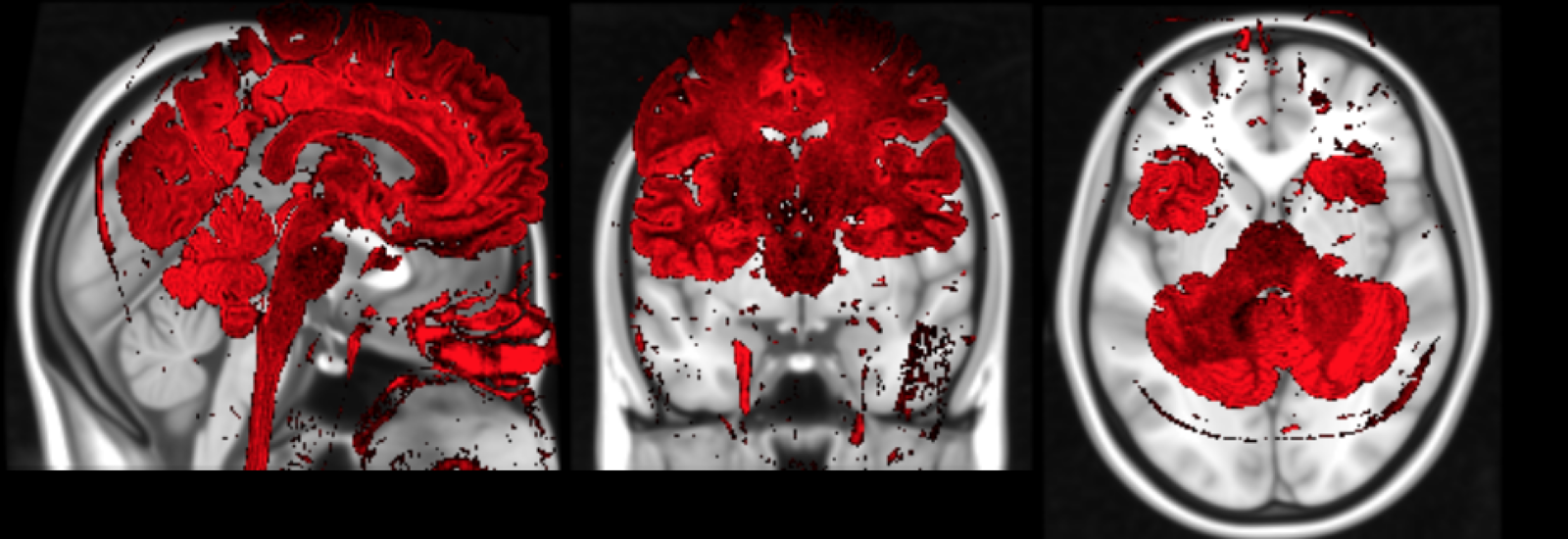
1. Introduction
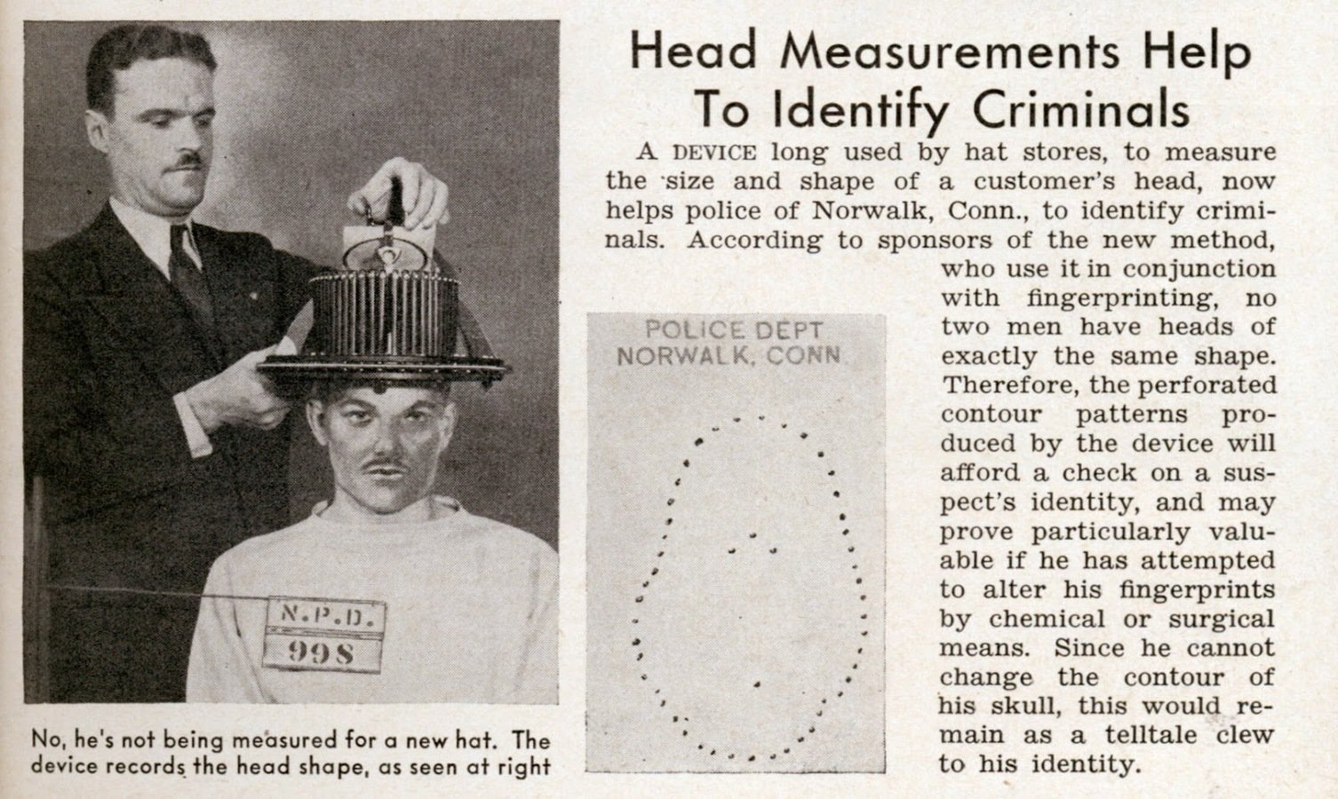
One of the first brain measurement...
A modern neurological study aims to relate several biomarkers from different sources in order to explain the illness evolution improve prognostic accuracy and optimize the treatment.
A modern research group can have at disposal:
- clinical,
- imaging,
- neuropsychological,
- liquor biomarkers
Neuroimaging offers a fecund source of biomarkers
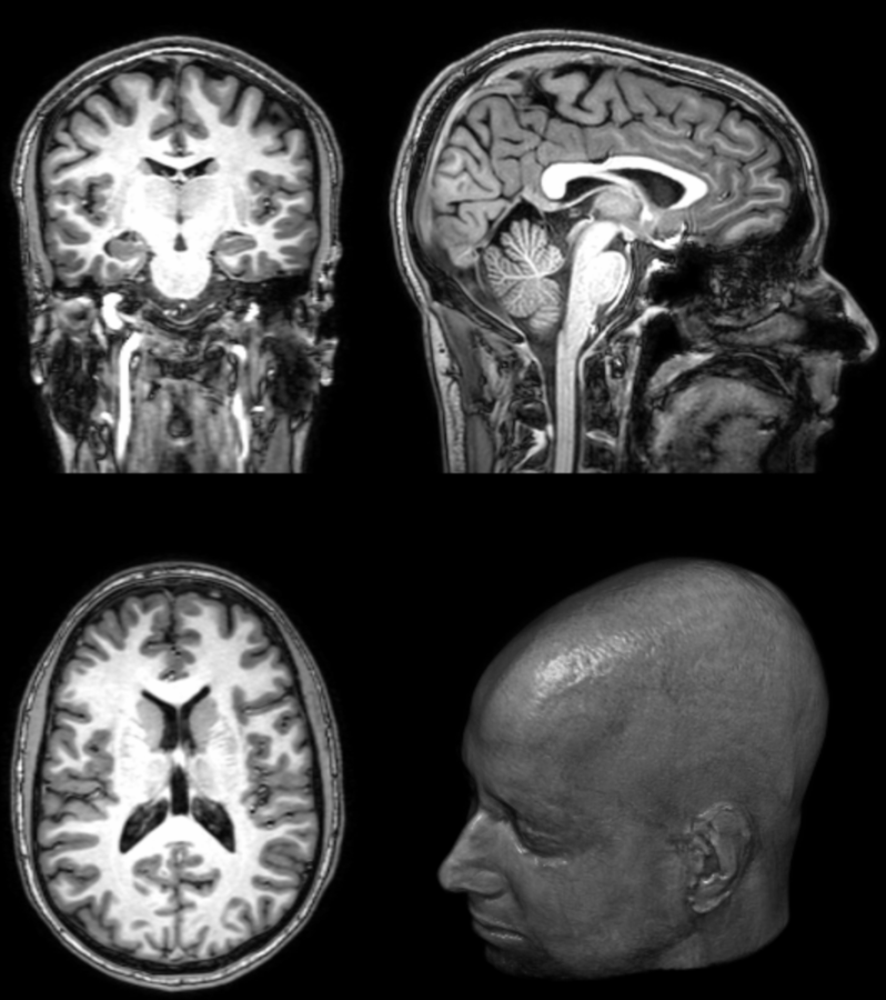
Computing biomarkers from neuroimaging sources can be time-consuming, also because an increasing number of images can be available from a single patient.
For instance, a study involving
- three 3D MRI images
- two 2D MRI sequences
- one dynamic brain PET
of 50 patients occupy more than 2Tb of disk space.
Hence there is need of improving the speed without loss of accuracy whenever possible.
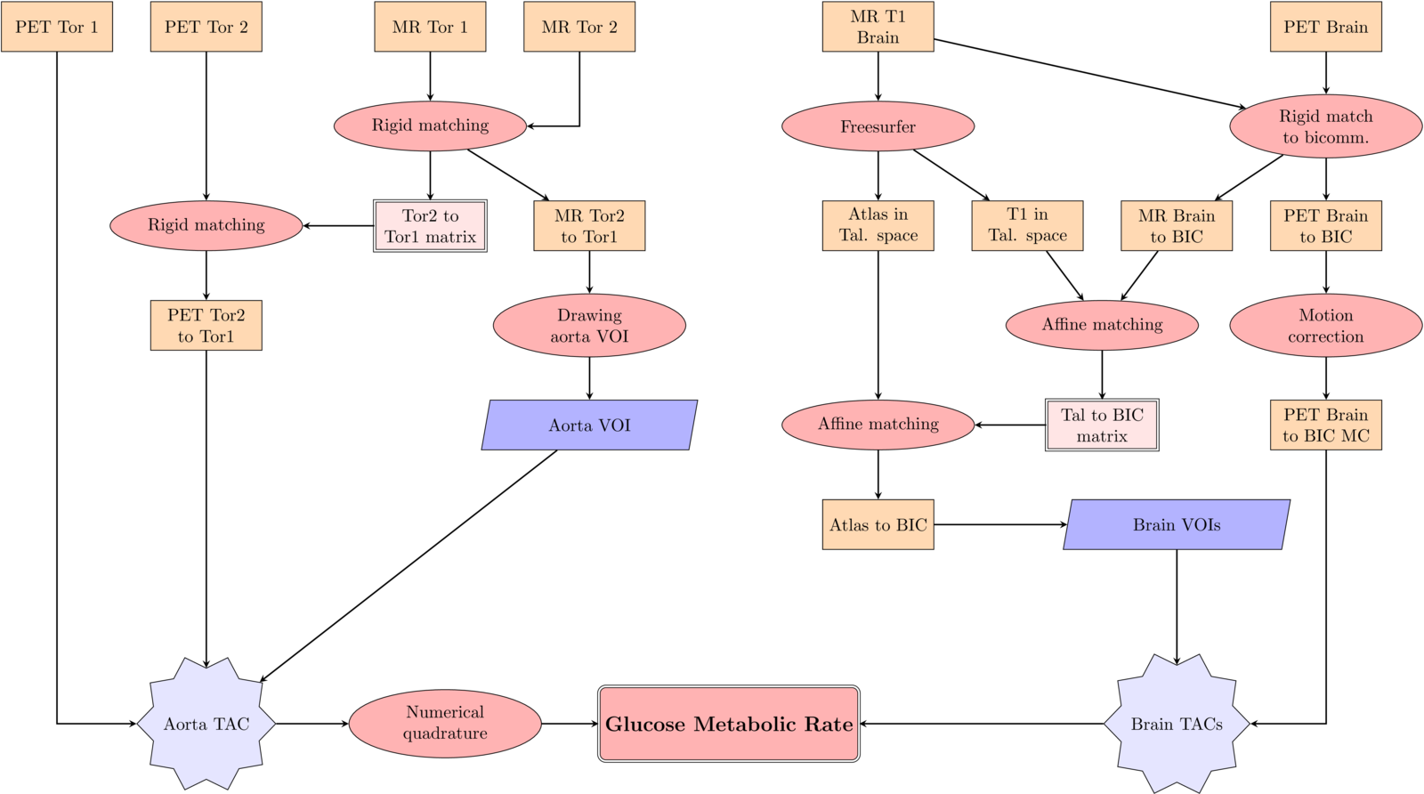
2. Common use algorithms & pipelines
1. Registration (rigid, affine, nonlinear)
2. Correction (Bias Field, Lesion Filling,
Motion Correction, PVC)
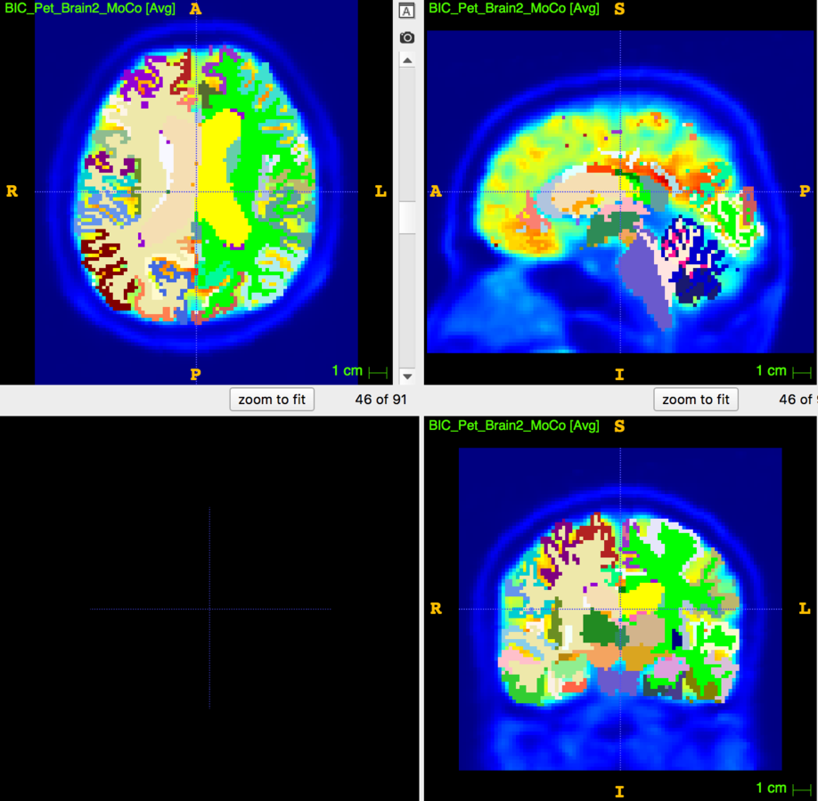
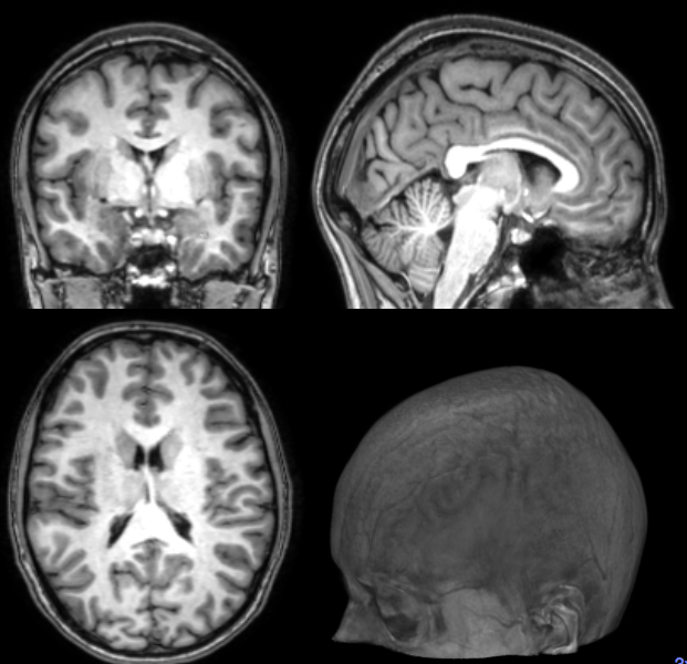
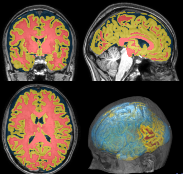
3. Segmentation (Manual, Template-based)
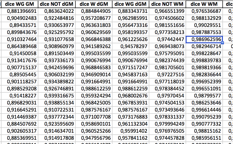
4. Measurement (mean, std over VOIs)
Registration
Correction
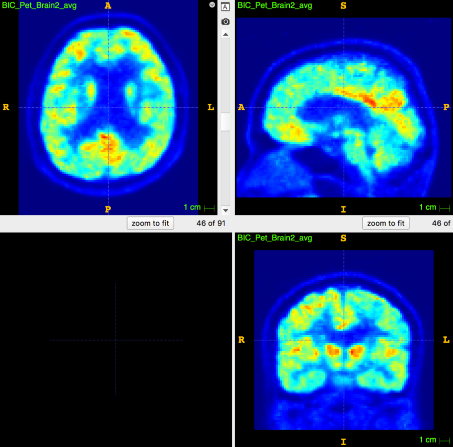
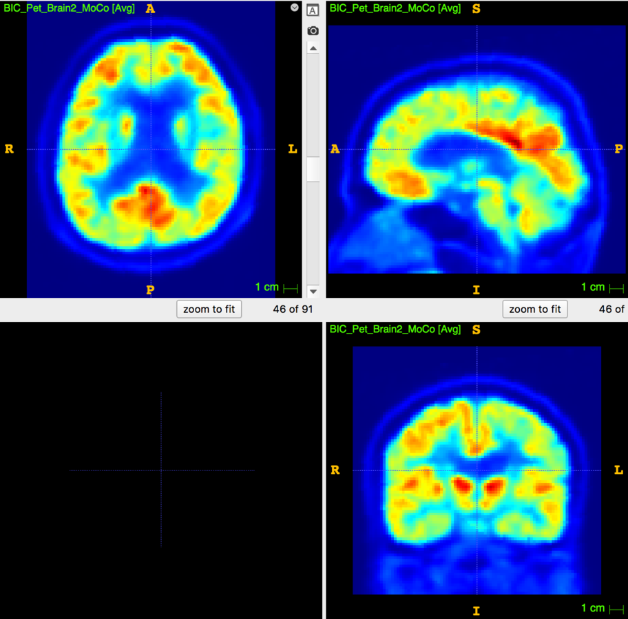
Motion Correction
Correction
Partial Volume Correction
Segmentation

Measurements
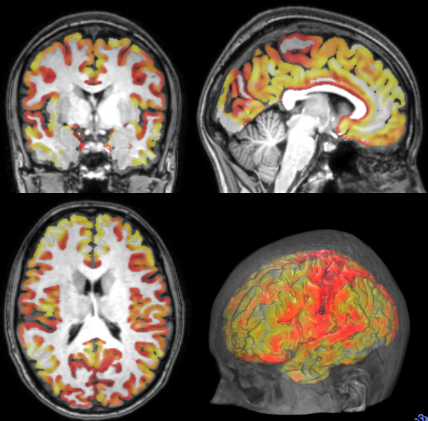
Cortical Thickness Estimation
Pipelining
3. Image Registration
What are we doing?
where D is an appropriate distance (or pseudo-distance).
Say that the image I is represented by a function
I : \Omega \subseteq \mathbb{R}^3 \longrightarrow \mathbb{R}
and the reference image is R we look for a function
f:\mathbb{R}^3\longrightarrow \mathbb{R}^3
\arg\min_{f} \mathcal{D}[I(f(x)),R(x)]
such that
Considering linear tranformation
f(x)=A⋅x+b
| DOF | Geom.meaning | A | det(A) |
|---|---|---|---|
| 3 | traslation | Identity | 1 |
| 6 | rototranslation | R s.t. det(R)=1 | 1 |
| 7 | homothety | aR, a>0 | a |
| 9 | similitude | diag(a,b,c)⋅R | abc |
| 12 | affinity | any s.t. det(R)≠0 | ≠0 |
The optimal transformation is found iteratively
Otherwise the transformation is called nonlinear
Speed it up
A good way of improving the convergence of this iterative method is to downsample the input image by a factor n and use the matrix as a initial guess for the next step.
# sample python code
# input image I, reference R
# functions `register' and `apply' are user-defined

from skimage.transform import downscale_local_mean

for in n [4,3,2,1]:
    II=downscale_local_mean(I,(n,n,n))
    I_out,mat_out=register(II,R,"affine",maxit=50,tol=1.e-5)
    I=apply(mat_out,I)
In python
One can use wrappers (as nipype)...but there is a pure-python registration routine inside nipy!
import numpy as np
import nibabel as nib
import nipy.algorithms.registration as nar
import sys
in_path=sys.argv[1]; ref_path=sys.argv[2]
IN=nib.load(in_path); REF=nib.load(ref_path)
#registration initialization
register_obj = nar.HistogramRegistration(from_img = IN, to_img = REF,\
similarity='crl1',interp=tri,renormalize=True)
#compute the optimal tranformation
transform = register_obj.optimize('affine', optimizer='bfgs',xtol = 1e-4,\
ftol = 1e-4,gtol = 1e-4,maxiter= 70)
#apply it
resampled = nar.resample(IN, transform, OUT)
#output the result
New=nib.Nifti1Image(resampled,header=IN.header,affine=REF.affine)
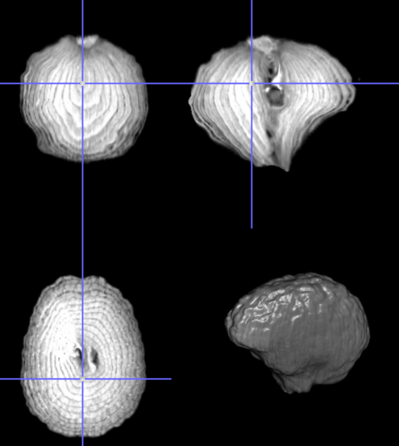
nib.save(New,sys.argv[3])Some funny example
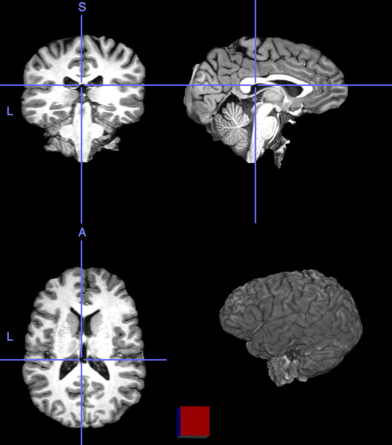
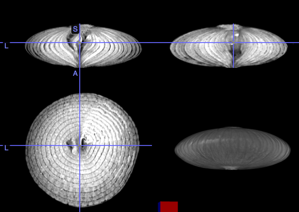
My brain is the reference, the onion the input image
Rigid transformation
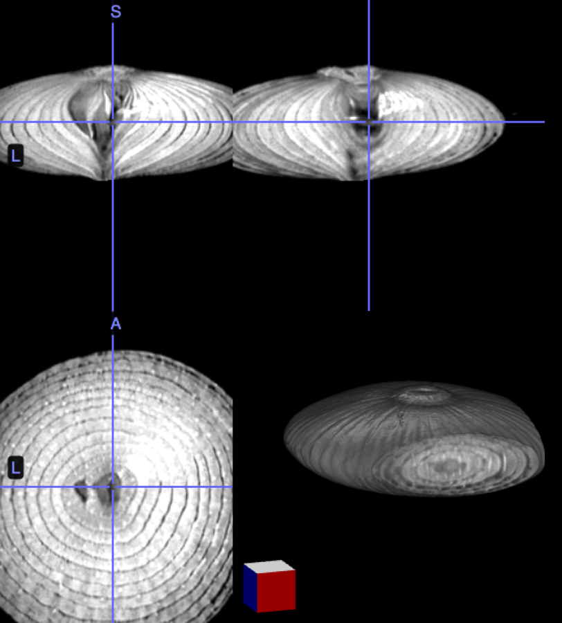
Affine transformation
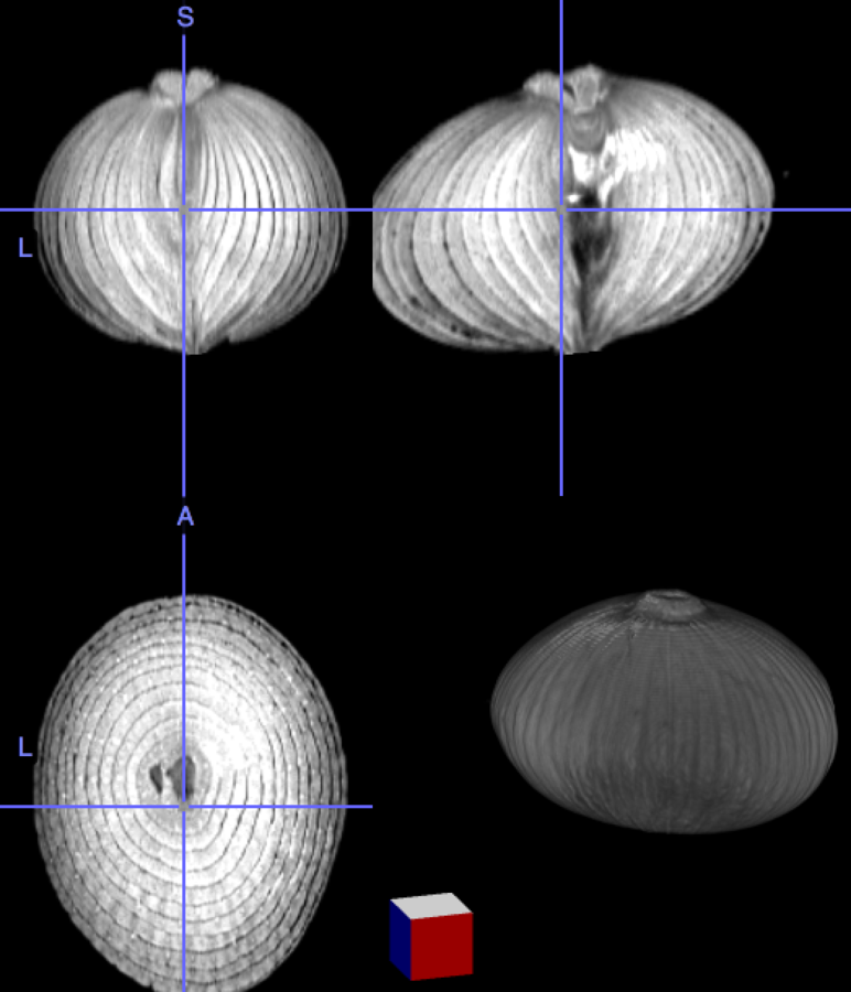
Nonlinear transformation
4. Patlak plot in PET/MRI
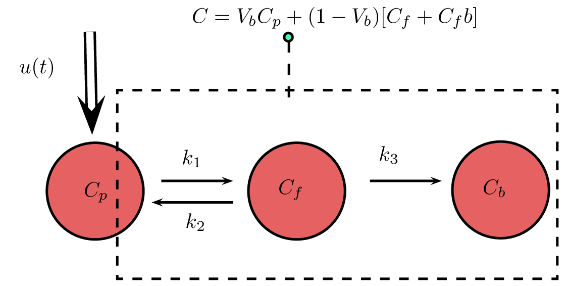
Sokoloff model for 18F-Fdg PET
Patlak plot method:
\frac{C(t)}{C_p(t)}=K \frac{\int_{0}^{t}C_p (\tau)\,d\tau}{C_p(t)} + V_b
K=\frac{k_{1}k_{3}}{k_{2}+k_{3}}
is proportional to the absolute Metabolic Rate
We can find K by linear fit
y=K x + b
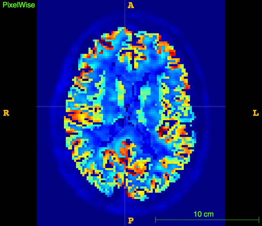
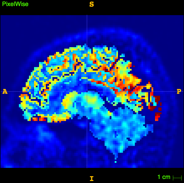
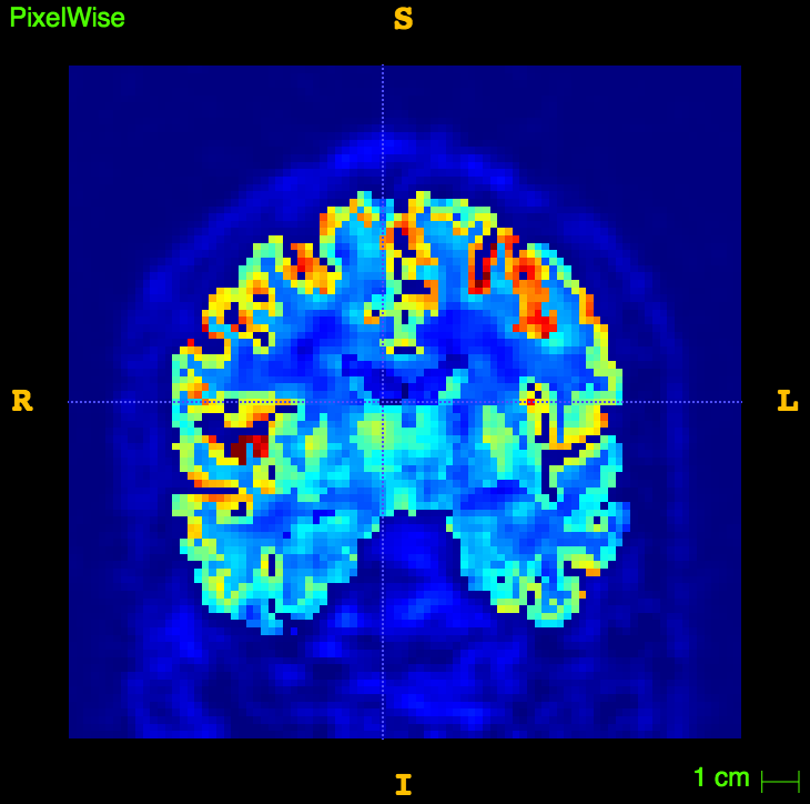
Speed it up
In the case of voxel-based Patlak, if you think about computing the result for each voxel in a (say) 128x128x128 image
for i in voxel:
    C,Cp,int_Cp=get_counts_voxel(i)
    X=int_Cp/Cp
    Y=C/Cp
    slope, intercept, r_value, p_value, std_err = stats.linregress(np.array(XX),np.array(YY))
You are going to have a bad time...
Solution: exploit the closed form of linear regression
\left( X , 1 \right) \cdot \left( \begin{array}{c} K \\ V_b \end{array} \right)=Y
Normal equations are
\left(\begin{array}{c c} X \cdot X^T & sum(X)\\ sum(X) & n \end{array} \right) \left(\begin{array}{c} K \\ V_b \end{array} \right) = \left(\begin{array}{c} X \cdot Y^t\\ sum(Y)\end{array} \right)
The solution of the system is
K = \frac{n X\cdot Y^T - sum(X)sum(Y)}{n X\cdot X^T - sum(X)sum(X)}
V_b = \frac{sum(X)}{n} - K \frac{sum(Y)}{n}
Which can be also applied if Y is a matrix containing all the voxel values over the time!
This will speed up the algorithm as the matrix multiplication is implemented in parallel in numpy
for i in voxel:
    C,Cp,int_Cp=get_counts_voxel(i)
    #save in matrix Y, X is a vector
    Y[:i]=C/Cp
X=int_Cp/Cp
n=X.shape[0]
Slope=(n*np.dot(XX,YY.T)-np.sum(XX)*np.sum(YY,1))/
        (n*np.dot(XX,XX.T)-np.sum(XX)*np.sum(XX))
Intercept=(np.sum(YY,1)/n)-Slope*(np.sum(XX/n))
In python:
before:
after:
for i in voxel:
C,Cp,int_Cp=get_counts_voxel(i)
X=int_Cp/Cp
Y=C/Cp
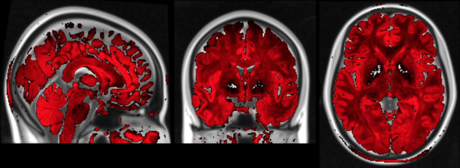
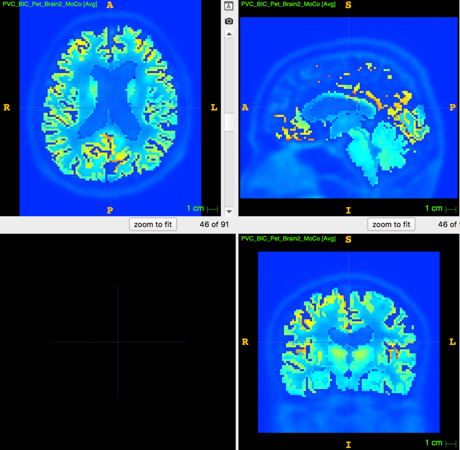
slope, intercept, r_value, p_value, std_err = stats.linregress(np.array(XX),np.array(YY))The resulting image
Thanks to....
MS Centre Padova
Nuclear Medicine Padova
Neurology Padova
Neuroradiology Unit Padova
all patients of course and...
... this audience for the attention!
Some References
- C Cobelli, D Foster, G Toffolo,Tracer kinetics in biomedical research, Springer, 2001.
- SR Das, BB Avants, M Grossman, JC Gee, Registration based cortical thickness measurement, Neuroimage. 2009
- CL Epstein, ntroduction to the mathematics of Medical Imaging, Second Edition, Siam, 2008
-
TG Feeman, The mathematics of medical imaging: A beginners guide, Springer, 2010
- ME Juweid, OS Hoekstra, Positron Emission Tomography, Humana Press, 2011.
- CS Patlak, RG Blasberg, Graphical evaluation of blood-to-brain transfer constants from multiple-time uptake data. Generalizations, Journal of Cerebral Blood Flow and Metabolism, 1985.
Data Analysis in MRI and PET/MRI Neuroimaging
By davide poggiali
Data Analysis in MRI and PET/MRI Neuroimaging
schei&paura? mai avui


