Fake Nodes approximation for Magnetic Particle Imaging

Stefano De Marchi, Wolfgang Erb, Francesco Marchetti,
Elisa Francomano, Emma Perracchione, Davide Poggiali

D. Poggiali, postDoc
MELECON 2020
Summary:
- Reconstruction in MPI
- Fake Nodes interpolation
- Numerical experiments
- Results and future works
Slides are available online
http://dpoggiali.altervista.org
to check out other work of mine.
1. Reconstruction in MPI
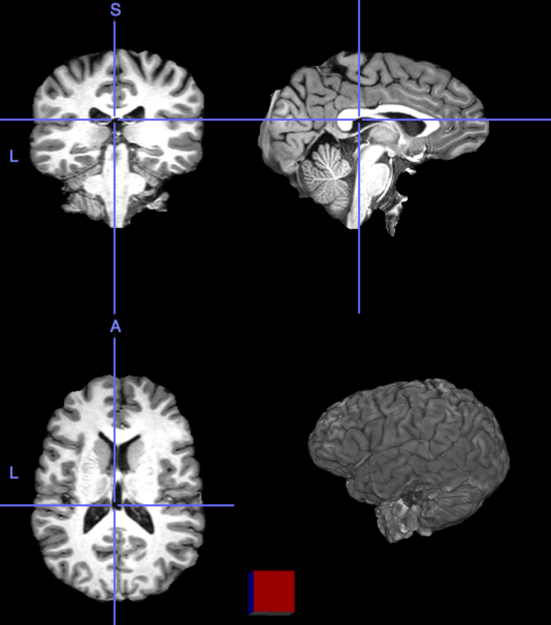
Magnetic Particle Imaging (MPI) is a tracer-based tomographic technique of recent development. MPI systems detect the spatial distribution of superparamagnetic nanoparticle tracers injected in the body.
Image acquisition in MPI is performed by generating a magnetic Field Free Point (FFP), moving along a chosen curve \(\gamma(t)\) and inducing a measurable voltage signal in a receive coil.
The scattered data obtained from this signal acquisition process can then be interpolated and evaluated over a regular grid to get a human-readable image; we will refer to this interpolation process as reconstruction.
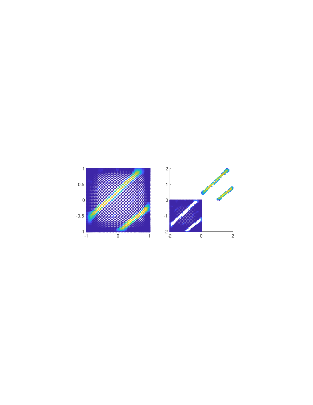
Commonly-used trajectories in MPI are Lissajous curves
\gamma(t)= \left( \cos (n_2t ), \, \cos \left( n_1 t - \frac{\epsilon-1}{2n_2}\pi \right) \right) \\
t \in [0, 2\pi], \; \epsilon \in \{ 1,2 \}, \; n_1, n_2 \in \mathbb{N}
\mathrm{LS} = \left\{\gamma\left(\frac{\pi k}{\epsilon n_1n_2}\right), \quad k=0,\ldots,2\epsilon n_1n_2-1 \right\}.
The sampling points are the so-called Lissajous nodes
2. Fake Nodes interpolation
Interpolation on Fake Nodes, or interpolation via Mapped Bases is a technique that applies to any interpolation method. It has shown in many cases the ability of obtaining a better interpolation without getting new samples.
This means that, provided that the original nodes are a sufficient sample of the given signal, it can be possible in principle to provide a more stable or accurate interpolation.
Fake Nodes interpolation
In terms of code: suppose that you have a generic interpolation function ...
def my_fancy_interpolator(x,y,xx):
  .......
  .......
  return yy
def my_fancy_interpolator(x,y,xx):
  p = np.polyfit(x,y)
  yy = np.polyval(p,xx)
  return yy
instead of calling the function directly you define a mapping function S and interpolate over the fake nodes S(x)
f = lambda x: np.log(x**2+1)
x = np.linspace(-1,1,10)
y = f(x)
xx = np.linspace(-1,1,100)


yy = my_fancy_interpolator(x,y,xx)
f = lambda x: np.log(x**2+1)
x = np.linspace(-1,1,10)
y = f(x)
xx = np.linspace(-1,1,100)
S = lambda x: -np.cos(np.pi * .5 * (x+1))
yy = my_fancy_interpolator(S(x),y,S(xx))In other words, given a function
f: \Omega \subseteq \mathbb{R}^d \longrightarrow \mathbb{R}\;\;\;\;\; {d \in \mathbb{N}},
a set of distinct nodes
X = \{ x_0, \dots, x_N\} \subset \Omega,
and a set of basis functions
\mathcal{B} = \{ b_i: \Omega \longrightarrow \mathbb{R} \}_{i = 0, \ldots, N}
The interpolant is given by a function
\displaystyle \mathcal{P}(\bm{x}) = \sum_{i=0}^{N} c_i b_i(\bm{x})
s.t.
\mathcal{P}(\bm{x}_i)=y_i:=f(\bm{x}_i) \;\;\forall i
\mathcal{B} = \{ b_i \circ S: \Omega \longrightarrow \mathbb{R}^d \}_{i = 0, \ldots, N}
\displaystyle \mathcal{R}^s(\bm{x}) = \sum_{i=0}^{N} c_i b_i(S(\bm{x}))
\mathcal{R}^s(\bm{x}_i)=y_i:=f(\bm{x}_i) \;\;\forall i
This process can be seen equivalently as:
1. Interpolation over the mapped basis
\[\mathcal{B}^s = \{b_i \circ S \}_{i=0, \dots, N}.\]
2. Interpolation over the original basis \(\mathcal{B}\) of a function \(g: S(\Omega) \longrightarrow\mathbb{R}\)
at the fake nodes
\[S(X) = \{S(x_i) \}_{i=0, \dots, N}.\]
\(g\in C^s\) must satisfy \(g(S(x_i)) = f(x_i)\;\;\forall i\).
If \(\mathcal{P} \approx g \) on \(S(X)\) with the original basis,
then \(\mathcal{R}^s = \mathcal{P} \circ S \approx f \) on \(X\)
3. Numerical experiments
A set of simulated MPI data whose ground truth is known has been generated, with parameters \(n_1 = 33, n_2 = 32, \epsilon=2\). Reconstruction has been performed on a 201x201 equispaced grid with different interpolation methods. Results have been compared to the ground truth.
Bivariate polynomial interpolation:
\(\mathcal{B} = \left \lbrace x_1^i x_2^j \right|\left. i,j = 0,\dots,K\text{ s.t. } i+j\leq K \right\rbrace\)
we used least-squares approximation with \(K=21\).
RBF interpolation:
\(\mathcal{B} = \left \lbrace K(\cdot, \bm{x}_i) \right\rbrace_{i = 0,\dots,N}.\)
being \(K(\cdot, \bm{x}_i) = \varphi(\|\cdot - \bm{x}_i\|_2)\) a kernel function.
we choose the Matérn functions of different regularities:
- \(\varphi_0(r)=\exp(-r) \in C^0\)
- \( \varphi_2(r)=\exp(-r)(1+r) \in C^2\)
- \(\varphi_4(r)=\exp(-r)(3 + 3r + r^2 ) \in C^4\)
- \(\varphi_6(r)=\exp(-r)(15 + 15r + 6r^2) \in C^6\)
\displaystyle S(x) = x + \sum_{k=1}^m \alpha_k \chi_{\Gamma_k}(x)
\alpha_k \coloneqq k (a,a)\;\;\; a>diam(\Omega)
Since our signal is discontinuous, its reconstruction will be affected by Gibbs phenomenon. To prevent this effect we used Fake Nodes interpolation with mapping \(S\) chosen as
being \(\Gamma_k\) the non-overlapping sets given by the segmentation of the image.
Symmetrized Kullbak-Leibner Divergence has been used for performance comparison.
where the Kullbak-Leibner Divergence is defined as
SKL(A,I) = KL(A,I) + KL(I,A)
KL(v,w) = \displaystyle\frac{\displaystyle\sum_{i=1}^{K} w_i \log\left(\frac{v_i}{w_i}\right)}{K}
4. Results and future works:

Polynomial approximation (left) and polynomial+Fake Nodes (right)
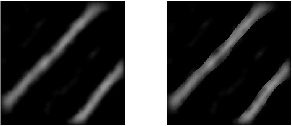
RBF \(C^0\) interpolation (left) and Fake-RBF \(C^0\) (right)
| Method | SKL (smaller is better) |
|---|---|
| Polynomial | 1.3581 |
| Fake-Polynomial | 0.6424 |
| RBF C⁰ | 0.7369 |
| Fake-RBF C⁰ | 0.6833 |
| RBF C² | 0.7947 |
| Fake-RBF C² | 0.8117 |
| RBF C⁴ | 0.8050 |
| Fake-RBF C⁴ | 0.9137 |
| RBF C⁶ | 1.0779 |
| Fake-RBF C⁶ | 1.0154 |
Future works:
Fake Nodes interpolation can be further investigated.
MPI reconstruction:
- Other RBF with different shape parameters,
- kernel Moving Least Squares.
Other bio-medical applications:
- image denoising,
- resolution approximation of an imaging system,
- MEG/EEG reconstruction.
References
[1] J P. Berrut, S. De Marchi, G. Elefante, F. Marchetti, Treating the Gibbs phenomenon in barycentric rational interpolation and approximation via the S-Gibbs algorithm. Applied Math. Letters, 2020.
[2] W. Erb, Bivariate Lagrange interpolation at the node points of Lissajous curves - the degenerate case, Appl. Math. Comput. 2016
[3] S. De Marchi, W. Erb, F. Marchetti, Lissajous sampling and spectral filtering in MPI applications: the reconstruction algorithm for reducing the Gibbs phenomenon, 2017 International Conference on Sampling Theory and Applications (SampTA), Tallin (2017).
[4] S. De Marchi, F. Marchetti, E. Perracchione, D. Poggiali, Polynomial interpolation via mapped bases without resampling, JCAM 2020.
[5] S. De Marchi, W. Erb, F. Marchetti, E. Perracchione, M. Rossini, Shape-Driven Interpolation with Discontinuous Kernels: Error Analysis, Edge Extraction and Applications in MPI, SIAM Sci. Comput. 2020
Thank you for your attention!
MELECON2020
By davide poggiali
MELECON2020
Money and fear? Never had either


