Audio Word2Vec: Unsupervised Learning of Audio Segment Representations using Sequence-to-sequence Autoencoder
Yu-An Chung, Chao-Chung Wu, Chia-Hao Shen, Hung-Yi Lee, Lin-Shan Lee
National Taiwan University
InterSpeech'16
Motivation
- Word2Vec has been shown to carry good semantic information of words in natural language processing.
- Q: Is it possible to do similar transformation of audio segments into vectors with fixed dimensionality?
- While Word2Vec carries semantic information of words, Audio Word2Vec carries phonetic structures of audio segments.
Background
- Representing variable-length audio segments by vectors with fixed dimensionality has been very useful for many speech applications.
- Speaker identification
- Audio emotion classification
- Spoken term detection (STD)
- Common approach
- Define feature vector in heuristic ways instead of learning from data.
Background
-
Recurrent Neural Network (RNN) approach
- Take audio segments as input, the corresponding word as target (supervised).
- The output of last few hidden layers can be taken as the representation of the input segment.
- Pros: Able to handle variable-length input.
- Cons: Labeled data is required.
Background
-
Autoencoder approach
- Take audio segments both as input and output (unsupervised).
- Map input segment to a vector with reduced dimensionality and reconstruct the vector back to the original input.
- The output of hidden layer can be taken as the representation of the input segment.
- Pros: No Labeled data is required.
- Cons: Unable to handle variable-length input.
Background
-
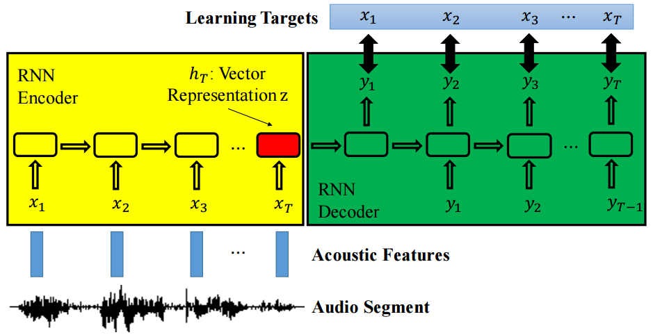
Sequence-to-sequence Autoencoder (SA) approach
- Take audio segments both as input and output (unsupervised).
- One RNN encoder: Encode the input sequence into a fixed length representation.
- One RNN decoder: Decode this input sequence out of that representation.
- This approach has already been applied in NLP and video processing, but not yet in speech signals.
- Pros: Able to handle variable-length input and no labeld data is required.
Proposed Approach
- Recurrent Neural Network (RNN)
- Given a sequence , update hidden state according to current input and the previous hidden state .
- The hidden state acts as an internal memory at time t that enables the network to capture dynamic temporal information.
- Since RNN does not seem to learn long-term dependencies, LSTM units are developed to replace the neurons.
x = (x_1, x_2, ..., x_T)
x=(x1,x2,...,xT)
h_t
ht
x_t
xt
h_{t-1}
ht−1
h_t
ht
Proposed Approach
- RNN Encoder-Decoder framework
- Consists of one RNN encoder and one RNN decoder.
- RNN encoder reads the input sequence and update the hidden state .
- RNN decoder takes hidden state and generate the output sequence .
- The length of input sequence T and output sequence T' can be different.
x = (x_1, x_2, ..., x_T)
x=(x1,x2,...,xT)
h_t
ht
h_t
ht
y = (y_1, y_2, ..., y_{T'})
y=(y1,y2,...,yT′)
Proposed Approach
-
Sequence-to-sequence Autoencoder (SA)
- Set RNN encoder-decoder framework's target sequence to be the same as input sequence.
-
Thus the objective function becomes the reconstruction error.
- The fixed-length vector representation will be a meaningful representation since the input sequence can be reconstructed from it by the RNN Decoder.
\sum\limits_{t=1}^T \lVert x_t-y_t \rVert^2
t=1∑T∥xt−yt∥2
Proposed Approach
-
Denoising Sequence-to-sequence Autoencoder (DSA)
- Randomly add some noise to the input acoustic feature sequence to make the learned representation more robust.
- DSA is expected to generate the output y closest to the original x based on the corrupted .
- This idea comes from the so-called denoising autoencoder.
\tilde{x}
x~
Example Application
-
Query-by-example STD
- Locate the occurrence regions of the input spoken query term in a large spoken archive without speech recognition.
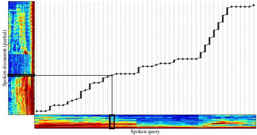
- Previous approach: Dynamic Time Warping (DTW)
- An algorithm for measuring similarity between two temporal sequences which may vary in speed.
- High computational cost.
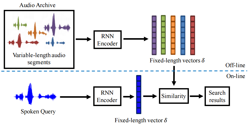
Cosine similarity
Experiments
- Dataset: LibriSpeech corpus
- A corpus of approximately 1000 hours of 16kHz read English speech.
- Training: 5.4 hours dev-clean (40 speakers)
- Testing: 5.4 hours test-clean (Different 40 speakers)
Experiments
-
Experiment settings
- Both training and testing are segmented by word boundaries.
- Only the beginning 13-dim of MFCC vector is used.
- Take k=100 for the representation's dimensionality.
- Zero-masking technique is used to generate noisy input sequences in DSA.
- Totally 5557 queries were made in testing set.
- Evaluation metric: Mean Average Precision (MAP)
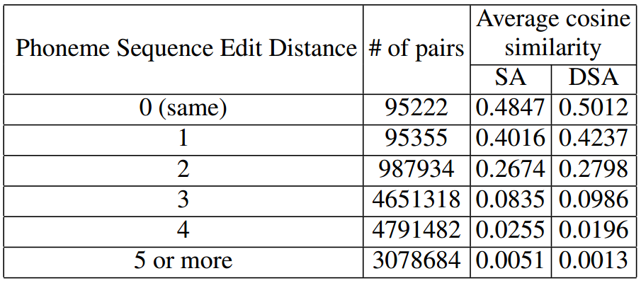
The minimum # of operations required to transform one string to another.
Observations
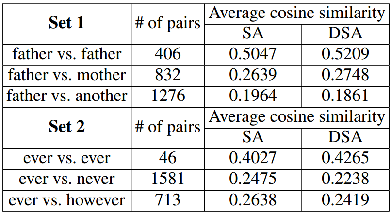
- 2 segments for words with larger phoneme sequence edit distances have obviously smaller cosine similarity in average.
- SA and DSA can even very clearly distinguish those word segments with only one different phoneme.
- The cosine similarity is a little bit small since even if two audio segments are exactly the same, they can have completely different acoustic realizations.
- DSA outperforms SA.
Observations
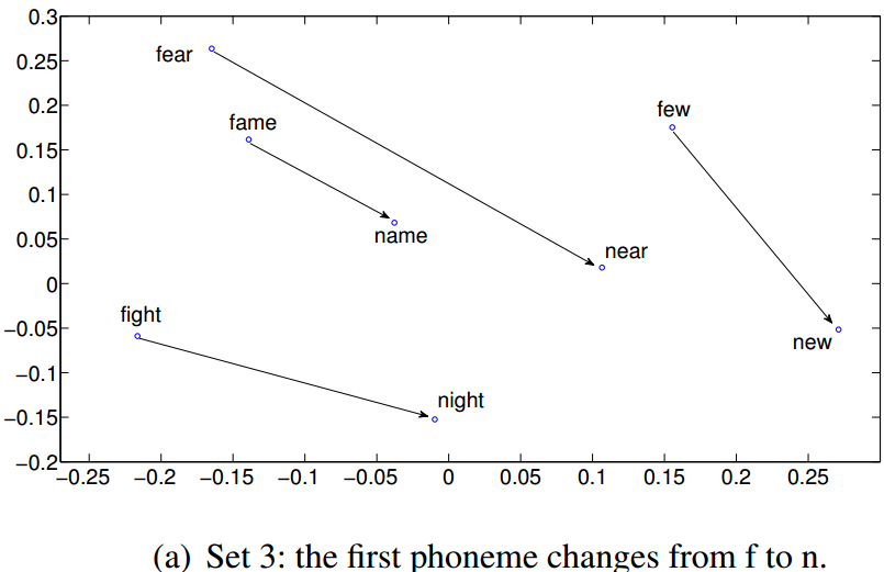
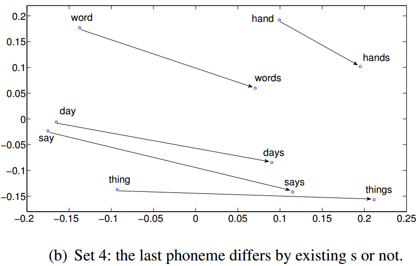
- It may be possible that the last few acoustic features dominate the vector representation, and as a result those words with the same suffixes are hard to be distinguished by the learned representations.
- However, these results show that although SA or DSA read the acoustic signals sequentially, words with the same suffix are still clearly distinguishable.
Experiments
- 2 baselines
- Frame-based DTW
- Adopt vanilla version of DTW.
- The frame-level distance is computed using Euclidean distance.
- Frame-based DTW
Experiments
- 2 baselines
- Naive Encoder (NE)
- Divide the input sequence into m segments with length of .
- Average each segment vectors into one single 13-dim vector.
- Concatenate all m average vectors to form one -dim vector.
- Naive Encoder (NE)
\frac{T}{m}
mT
13 \times m
13×m
Observations
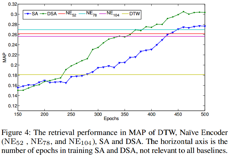
- Besides DTW which computes the distance between audio segments directly, all other approaches map the variable-length audio segments to fixed-length vectors for similarity evaluation.
- DTW has a poor performance.
- Only the vanilla version was used.
- The averaging process in NE may smooth some of the local signal variations which may cause disturbances in DTW.
Conclusions
- The author proposed 2 unsupervised approaches which combines RNN and autoencoder to obtain fixed-length vector representations for audio segments.
- The proposed approach outperforms the state-of-the-arts method in real world applications, such as query-by-example STD.
[InterSpeech][2016][Audio Word2Vec: Unsupervised Learning of Audio Segment Representations using Sequence-to-sequence Autoencoder]
By dreamrecord
[InterSpeech][2016][Audio Word2Vec: Unsupervised Learning of Audio Segment Representations using Sequence-to-sequence Autoencoder]
- 317


