Matrix Factorization

IRLAB Workshop
Kuan-Hao, Liao
09,07,2016

Recommender Systems

• Modern Recommender Systems:
  Analyze patterns of user interest in products to provide personalized recommendations that suit a user’s taste.
• Strategies:
  Content Filtering and Collaborative Filtering

Content Filtering

• Create a profile for each user or product to characterize its nature.
  e.g. Movie: genre, actors, box office popularity, etc.
            User: demographic info.
• Require gathering external information that might not be available or easy to collect.

Collaborative Filtering

• Relies only on past user behavior.
  (Mostly the previous transactions or product ratings)
• Domain free comparing to Content Filtering.
• Cold start problem:
  Difficult to address new products and users.
• 2 primary areas of collaborative filtering:
  Neighborhood methods and Latent factor models

Neighborhood Methods

• Centered on computing the relationships
  between items or between users.
• User-oriented and Item-oriented
• A user's neighbors are other users that tend to make similar ratings on the same product.
• A product’s neighbors are other products that tend
  to get similar ratings when rated by the same user.

Latent Factor Models

• Map users and items to the same vector space with certain latent features.
• Latent features can even include uninterpretable ones.
• A user's preference can be modeled by the
  dot product of the movie’s and user’s latent factor vector.

Neutral on this 2 dims.
This item/user may not be well represented by this 2 dims.

Matrix Factorization Model

• The most successful realizations of latent factor models.
• Good accuracy, scalability, and flexibility
• Can apply both explicit feedbacks (sparse) and implicit feedbacks (dense)

Matrix Factorization Model

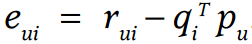
• The user-item interactions are modeled by                    
                                         where 
• Objective Function:
  Model directly the observed ratings only, while avoiding overfitting through a regularized model.

Matrix Factorization Model

• In comparison to Single Value Decomposition (SVD):
  - Usually rating matrix is sparse.
  - Conventional SVD assumes missing entries to be zeros, which is a poor assumption for rating matrix.

Learning Algorithms

• Stochastic Gradient Descent (SGD)
  Initialize user and item latent factor vectors randomly
  for t = 0, 1, ..., T
        (1) Randomly pick 1 known rating
        (2) Calculate Residual
        (3) Update user and item latent vector by gradient
  
   
• Pros: Efficient Execution

Learning Algorithms

• SGD has a better execution time than ALS.
• However, Parallelization can be applied to ALS.
  - All user latent factor vectors computations are independent of other user latent factor vectors.
  - All item latent factor vectors computations are independent of other item latent factor vectors.

Adding Bias

• Bias (Intercept):
  - User bias: Some users tend to give higher ratings than other users.
  - Item bias: Some items tend to receive higher ratings than other items.
• Biases can be modeled by
   

Adding Bias

• New rating with biases:
   
• The observed rating is broken down to 4 components:
  { Global average, Item bias, User bias, User-item interaction }
• This allows the 4 components to be explained independently.
• New Objective function:

Implementation

• GraphLab PowerGraph
  - Owned by Turi, Inc.
  - Written in C++
  - No longer updated
• LIBMF
  - Owned by C.-J. Lin, National Taiwan University
  - Written in C++
• scikit-learn NMF
  - Only for non-negative matrix factorization (NMF)
  - Supporting for Python interface

LIBMF

• Data format
  <row_idx> <col_idx> <value>
• Only integer index is supported, so manually indexing is required.
• Index starts from zero.

LIBMF

• Training
  - command
  mf-train [options] training_set_file model_file
  - options
  [-k]: number of latent factor dimensions
  [-t]: number of iterations

LIBMF

• Prediction
  - command
  mf-predict [options] test_file model_file output_file

loss function type

rating matrix's shape (m by n)

# latent factor dims

latent factor vectors of matrix P

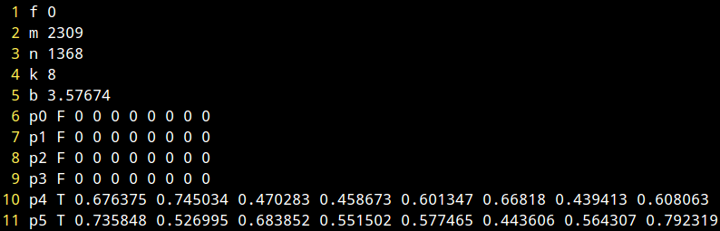
• Model file                                                                              
  
  

LIBMF