Electrostatics
The Electric Potential
Electrostatics
The Electric Potential
Learning Outcomes

Learn how to:
Calculate the electric potential at a given point in space due to
- a configuration of point charges.
- a "continuous" distribution of electric charges.
Relate the electric potential to
- the electric potential energy
- the electric field
Electrostatics
The Electric Potential
Walkthrough
Electrostatics
The Electric Charge
Charge Distribution

Electrostatics
Electric Charge
Charge Distributions
\lambda = dq / dl
Linear Charge Density
\sigma=dq / dA
Surface Charge Density
\rho=dq / dV
Volume Charge Density
\lambda_\text{\tiny uniform} = \frac{Q_\text{\tiny total}}{l_\text{\tiny total}}
\sigma\text{\tiny uniform} = \frac{Q_\text{\tiny total}}{A_\text{\tiny total}}
\rho\text{\tiny uniform} = \frac{Q_\text{\tiny total}}{V_\text{\tiny total}}
Electrostatics
Electric Charge
Point Charge
Charge distribution A
Charge distribution B
What do we mean by point charges?
\text{size$_\text{charge distribution}$}
\text{scale of analysis}
\lt\lt\lt
Electrostatics
The Electric Charge
... and the rest of the cast
Electrostatics
The influence & interaction of electric charges
The Cast
q
\vec{E}
V
\Phi
\vec{F}
U
potential
potential energy
field
force
charge
flux
influence
interaction
Electric ....
Electrostatics
The influence & interaction of electric charges
The Cast - relationship map
Electric ....
\vec{E}
V
\Phi
influence
interaction
\ \vec{E}=-\vec{\nabla} V\
\ \Delta V = -\int \vec{E}\cdot d\vec{s}\
\ \Phi = \int \vec{E}\cdot d\vec{A}\
\vec{F}
U
\ \vec{F}=-\vec{\nabla} U\
\ \Delta U = -\int \vec{F}\cdot d\vec{s}\
\ \vec{F} = q_0\ \vec{E}\
\ \vec{E} = \vec{F}/q_0\ \
\ U = q_0\ V\
\ V = U/q_0\ \
q
Electrostatics
The influence & interaction of electric charges
The Cast - relationship map
Electric ....
\vec{E}
V
\Phi
influence
interaction
\ \vec{E}=-\vec{\nabla} V\
\ \Delta V = -\int \vec{E}\cdot d\vec{s}\
\ \Phi = \int \vec{E}\cdot d\vec{A}\
\vec{F}
U
\ \vec{F}=-\vec{\nabla} U\
\ \Delta U = -\int \vec{F}\cdot d\vec{s}\
\ \vec{F} = q_0\ \vec{E}\
\ \vec{E} = \vec{F}/q_0\ \
\ U = q_0\ V\quad
\ V = U/q_0\ \
q
\Phi_g
influence
\ \Phi_g = \int \vec{g}\cdot d\vec{A}\
\vec{g}
gy
\ \vec{g}=-\vec{\nabla} (gy)\
\ \Delta V = \int \vec{g}\cdot d\vec{s}\
\vec{F}_g
mgy
interaction
\ \vec{F}=-\vec{\nabla} (mgy)\\
=-mg\hat j
\ \Delta U = -\int \vec{F}\cdot d\vec{s}\
m
\ \vec{F_g} = m\ \vec{g}\
\ \vec{g} = \vec{F_g}/m\ \
\ U_g = m\ V_g\
\ V_g = U_g/m\ \
gravitational....
analogus to
Electrostatics
The Electric Potential
conceptual overview
Electrostatics
The Electric Potential
conceptual overview
Follow along with [CQ] Electric Potential
Electrostatics
The Electric Potential
Conceptual overview
Electric Charges have an influence in their vicinity that we call the Electric Potential.
Perhaps you can think of it as a fictious glow surrounding each charge.
The "glow" at any point in space is the combined result of all the "glow" from the distribution of charges.
Electrostatics
The Electric Potential
Conceptual overview
The Electric Potential due to a point charge is proportional to the charge.
The Electric Potential due to a point charge is ...

inversely proportional to the distance from that charge.
The Electric Potential at some location due to a point electric charge depends on the material(s) in the region(s) separating the charge and that location.

Electrostatics
The Electric Potential
Conceptual overview
The Electric Potential due to a point charge is
V(r)=\frac{kq}{r}
given by ...
charge creating potential.
distance from the charge q to the point of interest P
material-dependent proportionality constant
k:
q:
r:
Electrostatics
The Electric Potential
Point-charge
V(r)=\frac{kq}{r}
\text{the Electric Potential due to a point-charge $q$ at some distance $r$}
Visualizingthe Electric Potential from a point-charge
Electrostatics
The Electric Potential
due to a point charge
Electrostatics
The Electric Potential
Point-charge
Video walkthrough this stack
Electrostatics
The Electric Potential
Point-charge
V(r)=\tfrac{1}{4\pi\epsilon}\frac{q}{r}
\text{the Electric Potential due to a point-charge $q$ at some distance $r$}
\text{permittivity}
\text{SI unit: Volt (V)}
\text{Volt}= \text{Joule / Coulomb}
\text{Scalar Quantity } (\pm)
\kappa : \text{relative permittivity (Dielectric Constant)}
\text{Permittivity of free space: } \epsilon_0=8.854\times10^{-12}\ C^2/Nm^2
\text{Absolute Permittivity (material dependent): } \epsilon = \kappa \epsilon_0
\text{In free space: } k=1/4\pi\epsilon_0 = 8.99\times10^{9}\ Nm^2/C^2
Electrostatics
The Electric Potential
Point-charge
V(r)=\tfrac{1}{4\pi\epsilon_0}\frac{q}{r}
\text{**Calculate the electric potential produced by}\\\text{ a point-charge of $3.0\mu C$ at a distance of 2.0mm}
=\tfrac{(8.99\times10^9 Nm^2/C^2) \ \times (3\times10^{-6} \ C)}{(2 \times10^{-3} m)}
=1.3\times10^7 V
Electrostatics
The Electric Potential
Point-charge
V=\tfrac{1}{4\pi\epsilon_0}\frac{q}{r}
Suppose that a point charge of 8.0nC is located at r_q=(0.50m, 1.5m) according to some 2D Cartesian coordinate system.
Calculate the electric potential produced by the charge at the shown locations P_1 and P_2.
x
y
0.50 m
=\tfrac{(8.99\times10^9 Nm^2/C^2) \ \times (8\times10^{-9} \ C)}{\sqrt{(6 \times0.5 m)^2+(2 \times0.5 m)^2})}
=23 V
=\tfrac{1}{4\pi\epsilon_0}\frac{q}{|\vec{r}_{P_1}-\vec{r_q}|}
P_1
P_2
=\tfrac{(8.99\times10^9 Nm^2/C^2) \ \times (8\times10^{-9} \ C)}{\sqrt{(2 \times0.5 m)^2+(-2 \times0.5 m)^2})}
=50 V
=\tfrac{1}{4\pi\epsilon_0}\frac{q}{|\vec{r}_{P_2}-\vec{r_q}|}
Electrostatics
The Electric Potential
Point-charge
V(r)=\tfrac{1}{4\pi\epsilon}\frac{q}{r}
Example:
In Bohr's model of the Hydrogen atom (1 proton + 1 electron), the electron orbits the proton in circular orbitals, whose radii are given by . Find an expression for the electric potential due to the proton at the location of the electron.and calculate for n=1. (known as the gorund state)

Electrostatics
The Electric Potential
due to a configuration of point charges
Electrostatics
The Electric Potential
Multiple point charges
V_\text{@ P}={\Large \Sigma}_{\tiny {i=1}} ^{\tiny N} \ \frac{k\ q_i}{r_i}
\text{The Net Electric Potential due to multiple point-charges }
q_1
q_2
q_N
\text{algebriac sum}
\text{the contribution due to $q_i$}
Electrostatics
The Electric Potential
Multiple point charges
V_\text{@ P}={\Large \Sigma}_{\tiny {i=1}} ^{\tiny N} \ \frac{k\ q_i}{r_i}
Electrostatics
The Electric Potential
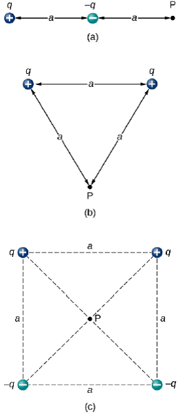
Multiple point charges
(a)
V_\text{@ P}={\Large \Sigma}_{\tiny {i=1}} ^{\tiny N} \ \frac{k\ q_i}{r_i}
=\frac{k\ (+q)}{2a}
+
\frac{k\ (-q)}{a}
=\frac{-kq}{2a}
(b)
V_\text{@ P}={\Large \Sigma}_{\tiny {i=1}} ^{\tiny N} \ \frac{k\ q_i}{r_i}
=\frac{k\ (+q)}{a}
+
\frac{k\ (+q)}{a}
=\frac{2kq}{a}
e.g. For each of the shown charge configurations, find an expression for the net Electric Potential at point P
(c)
V_\text{@ P}={\Large \Sigma}_{\tiny {i=1}} ^{\tiny N} \ \frac{k\ q_i}{r_i}
=\frac{k\ (+q)}{a/\sqrt{2}}
+
\frac{k\ (+q)}{a/\sqrt{2}}+\frac{k\ (-q)}{a/\sqrt{2}}
+
\frac{k\ (-q)}{a/\sqrt{2}}
=0
Electrostatics
The Electric Potential
Representation and Visualization
Electrostatics
The Electric Potential
Visualizing the Electric Potential
V_\text{@ P}={\Large \Sigma}_{\tiny {i=1}} ^{\tiny N} \ \frac{k\ q_i}{r_i}
Electrostatics
The Electric Potential
Visualizing the Electric Potential
V_\text{@ P}={\Large \Sigma}_{\tiny {i=1}} ^{\tiny N} \ \frac{k\ q_i}{r_i}
Electrostatics
The Electric Potential
Visualizingthe Electric Potential from a point-charge (1D)
Visualizing the Electric Potential
V_\text{@ P}={\Large \Sigma}_{\tiny {i=1}} ^{\tiny N} \ \frac{k\ q_i}{r_i}
Electrostatics
The Electric Potential
Equipotential Surfaces
Electrostatics
The Electric Potential
Equipotential Surfaces
The "landscape" analogy
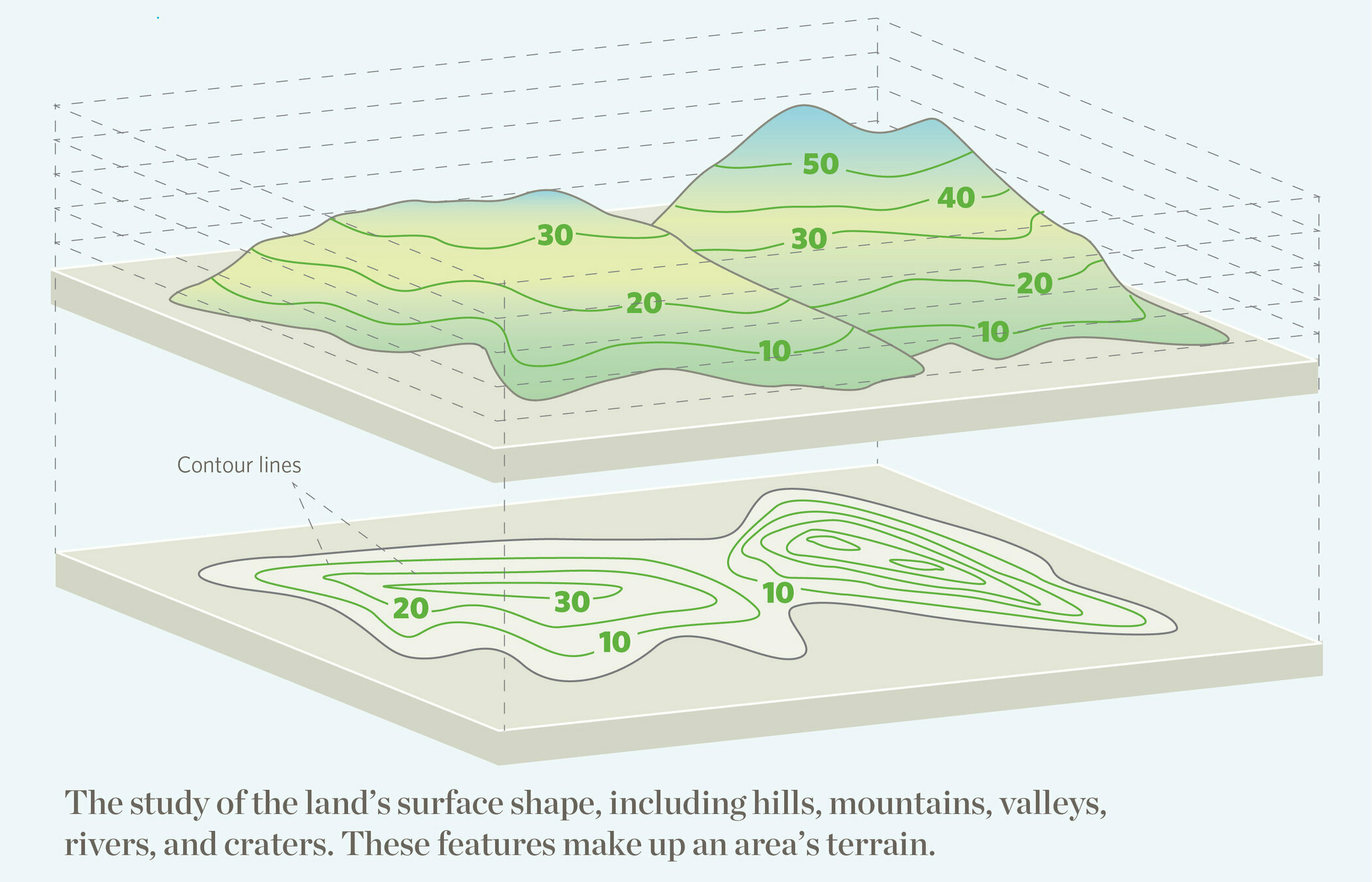
Electrostatics
The Electric Potential
Equipotential Surfaces
toggle between
3D view and Equipotential view
Vary the charges and their locations
Electrostatics
The Electric Potential
Equipotential Surfaces
In this simulation, the shown curves represent the intersection of the equipotential surfaces with the shown plan
use the pencil button on the cross-hairs tool.
Electrostatics
The Electric Potential
Equipotential Surfaces
In this simulation, the shown curves represent the intersection of the equipotential surfaces with the chosen plan
show different slices to investigate the whole 3D space
Electrostatics
The Electric Potential
Equipotential Surfaces
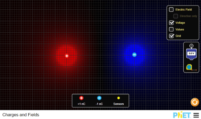
Mission:
- Map the electric potential "landscape" and compare to expected
- Investigate the average and local Electric Fields using the electric potential map.
- ...
Part I: Map the electric potential "landscape"
- Imagine an x-y coordinate system:
- Place a charge +2nC at x=-1.500+/- 0.005m and y=0.000+/-0.005m
- Place a charge -2nC at x=+1.500+/- 0.005m and y=0.000+/-0.005m
Electrostatics
The Electric Potential
Equipotential Surfaces
Electrostatics
The Electric Potential
The Potential Difference (aka Voltage)
Electrostatics
The Electric Potential
The Electric Potential Difference (aka Voltage)
\Delta V
\Delta V
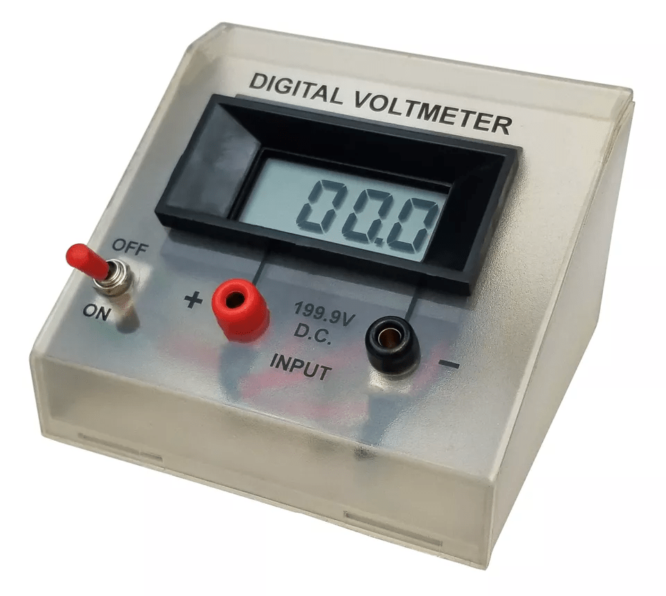
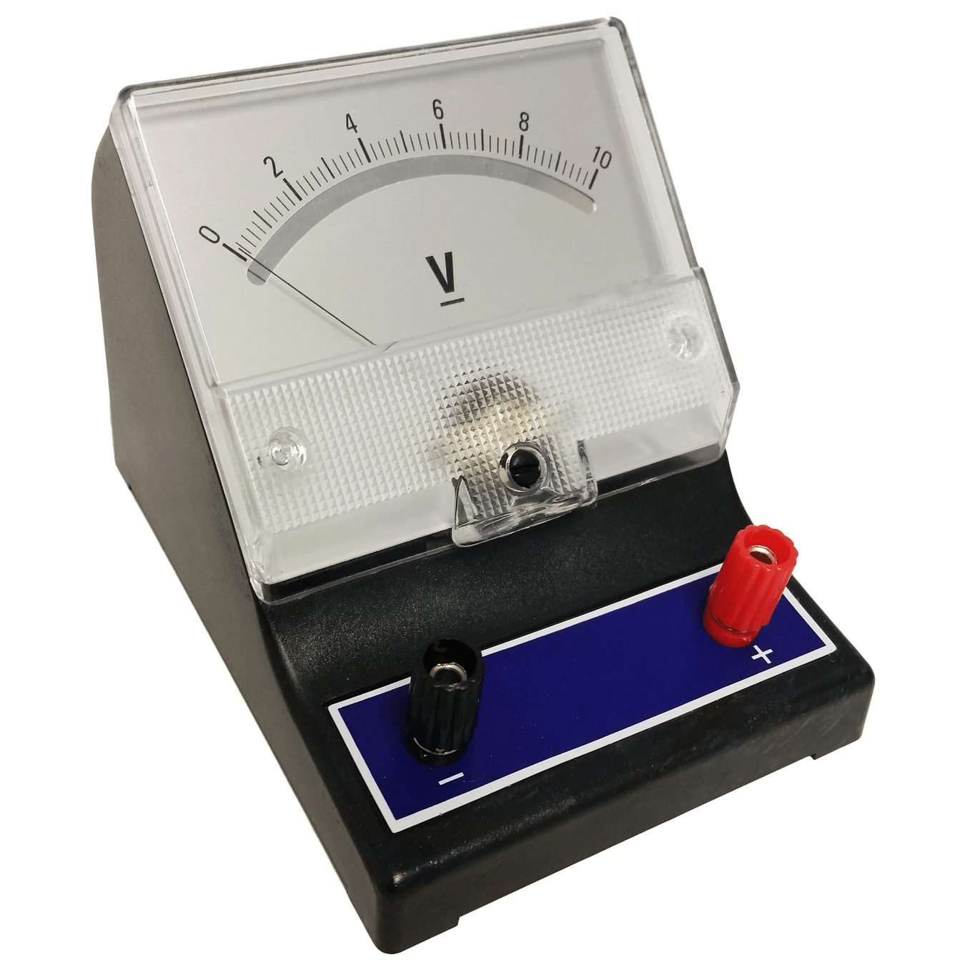
ANALOG VOLTMETER
The Instruments measure the electric potential difference between any two points in space.
Electrostatics
The Electric Potential
The Electric Potential Difference (aka Voltage)
\Delta V
\Delta V
ANALOG VOLTMETER
The Electric Potential is defined up to an arbitrary scalar shift
Therefore, it is the Electric Potential Difference that really matters
The Electric Potential Difference between any two points in space, A and B, is given by:
\Delta V= V_B-V_A
Electrostatics
The Electric Potential
and The Electric Potential Energy
Electrostatics
The Electric Potential
Relationship to the Electric Potential Energy
Video Walkthrough this stack
Electrostatics
V
influence at some location in space
interaction between charges
U
\ U = q_0\ V\
\ V = U/q_0\ \
The Electric Potential
Relationship to the Electric Potential Energy
Electric
Potential
Electric
Potential
Energy
Electrostatics
The Electric Potential
Relationship to the Electric Potential Energy
\text{P$_1$}
\text{P$_2$}

When a mass m is displaced between locations P1 to P2
\text{($m$ @ $P_1$)$\rightarrow$ ($m$ @ $P_2$)}
= m\ (gy{_2}-gy{_1})
The mass of the object being displaced
The difference between the gravitational potential at the two points due to Earth
Gravity analogy
\Delta U_g
The change in the Gravitational Potential Energy is given by:
= mgy{_2}-mgy{_1}
Electrostatics
The Electric Potential
relationship to the Electric Potential Energy
\Delta V
q_0\ (V_{@P_2}-V_{@P_1})
\Delta U_\text{($q_0$ @ $P_1$)$\rightarrow$ ($q_0$ @ $P_2$)}=
The change in the Electric Potential Energy as some charge q0 is transferred from point P1 to point P2
The amount of net charge being transferred
The Electric Potential Difference between points P1 and P2
SI units: Substituting for
the charge in Coulombs, and
the Electric Potential in Volts,
results in the Energy in Joules
Electrostatics
The Electric Potential
relationship to the Electric Potential Energy
\Delta V
\Delta U_\text{($q_0$ @ $P_1$)$\rightarrow$ ($q_0$ @ $P_2$)}= q_0\ (V_{@P_2}-V_{@P_1})
Electrostatics
The Electric Potential
and The Electric Field
Electrostatics
Video walkthrough this stack
The Electric Potential
Relationship to the Electric Field
Electrostatics
\vec{E}
V
The influence
of Electric Charges
The Electric Potential
Relationship to the Electric Field
\ \Delta V = \int \vec{E}\cdot d\vec{s}\
\ \vec{E}=-\vec{\nabla} V\
Electrostatics
The Electric Potential
Relationship to the Electric Field
The Electric Field ~ the slope of the Electric Potential
\Delta V
\Delta s
\Delta V
\Delta s
Electrostatics
The Electric Potential
Relationship to the Electric Field
\vec{E}
V
\ \vec{E}=-\vec{\nabla} V\
\Delta s
\Delta V
V_1
V_2
s_1
s_2
The average Electric Field
\vec{E}_\text{avg}=-\frac{~~~~~~~~}{~~~~~~~}\ \hat{s}
\Delta V
\Delta s
magnitude = Electric Potential Difference per unit length.
direction = from High potential to Low potential
V
s
Electrostatics
The Electric Potential
Relationship to the Electric Field
V
s
s_1
s_2
V_1
V_2
\Delta s
\Delta V
\vec{E}
V
\ \vec{E}=-\vec{\nabla} V\
s_3
\vec{E}=-\ \frac{~~~~~~}{~~~~~}\ \hat{s}
d V
d s
The local Electric Field
\ \vec{E}=-\vec{\nabla} V\
In higher dimensions
Math Interlude
Differential Calculus

\vec{\nabla} f{\small (r,\theta,\phi)}= \tfrac{\partial f}{\partial r}\ \hat{r}
+
\tfrac{1}{r}\tfrac{\partial f}{\partial \theta}\ \hat{\theta}
+
\tfrac{1}{r \sin\theta}\tfrac{\partial f}{\partial \phi}\ \hat{\phi}
Spherical Coordinates
\vec{\nabla} f{\small (x,y,z)}= \tfrac{\partial f}{\partial x}\ \hat{i}
+
\tfrac{\partial f}{\partial y}\ \hat{j}
+
\tfrac{\partial f}{\partial z}\ \hat{k}

Cartesian Coordinates
\vec{\nabla} f{\small (x,y,z)}= \tfrac{\partial f}{\partial x}\ \hat{i}
+
\tfrac{\partial f}{\partial y}\ \hat{j}
+
\tfrac{\partial f}{\partial z}\ \hat{k}
Cartesian Coordinates
h{\small (x,y,z)}= ay+b
\vec{\nabla} h{\small (x,y,z)}= \tfrac{\partial h}{\partial x}\ \hat{i}
+
\tfrac{\partial h}{\partial y}\ \hat{j}
+
\tfrac{\partial h}{\partial z}\ \hat{k}
= 0\ \hat{i}
~~+~
a\ \hat{j}
~~+~
0\ \hat{k}
f{\small (x,y,z)}= axy^2+x^2 z
\vec{\nabla} f{\small (x,y,z)}=
+
x^2\ \hat{k}
+2axy\ \hat{j}
(ay^2+2xz) \hat{i}
\tfrac{\partial f}{\partial x}\ \hat{i}
+
\tfrac{\partial f}{\partial y}\ \hat{j}
+
\tfrac{\partial f}{\partial z}\ \hat{k}
=
Math Interlude
Differential Calculus
\vec{\nabla} f{\small (r,\theta,\phi)}= \tfrac{\partial f}{\partial r}\ \hat{r}
+
\tfrac{1}{r}\tfrac{\partial f}{\partial \theta}\ \hat{\theta}
+
\tfrac{1}{r \sin\theta}\tfrac{\partial f}{\partial \phi}\ \hat{\phi}
Spherical Coordinates
Math Interlude
Differential Calculus
\vec{\nabla} f{\small (r,\theta,\phi)}=
\tfrac{\partial f}{\partial r}\ \hat{r}
+
\tfrac{1}{r}\tfrac{\partial f}{\partial \theta}\ \hat{\theta}
+
\tfrac{1}{r \sin\theta}\tfrac{\partial f}{\partial \phi}\ \hat{\phi}
{\small \sin\phi}\ \hat{r}
\small +0\ \hat{\theta}
=
-
\tfrac{r\cos\phi}{r \sin\theta}\ \hat{\phi}
\vec{\nabla} V{\small (r,\theta,\phi)}=
\tfrac{\partial V}{\partial r}\ \hat{r}
+
\tfrac{1}{r}\tfrac{\partial V}{\partial \theta}\ \hat{\theta}
+
\tfrac{1}{r \sin\theta}\tfrac{\partial V}{\partial \phi}\ \hat{\phi}
=
-\tfrac{kq}{r^2}\ \hat{r}
\small +0\ \hat{\theta}
\small +0\ \hat{\phi}
\vec{E}=\tfrac{kq}{r^2}\ \hat{r}
V=\tfrac{kq}{r}
\ \vec{E}=-\vec{\nabla} V\
For a point charge
f{\small (r,\theta,\phi)}= r \sin\phi
V{\small (r,\theta,\phi)}= \tfrac{kq}{r} + V_0
Electric Potential
By drmoussaphysics
Electric Potential
Introduction to electric potential