Deep Probabilistic Learning
Capturing Uncertainties with Deep Neural Networks

Francois Lanusse @EiffL
+ p(x) =


Before we dive in...
Let's talk about uncertainty
A Motivating Example: Probabilistic Linear Regression
From this excellent tutorial:
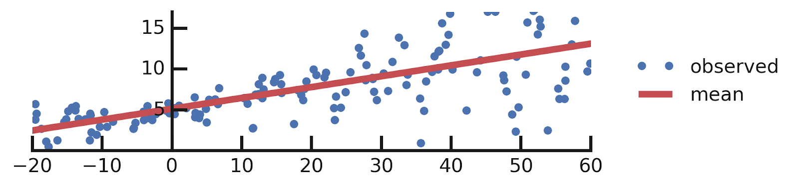
- Linear regression
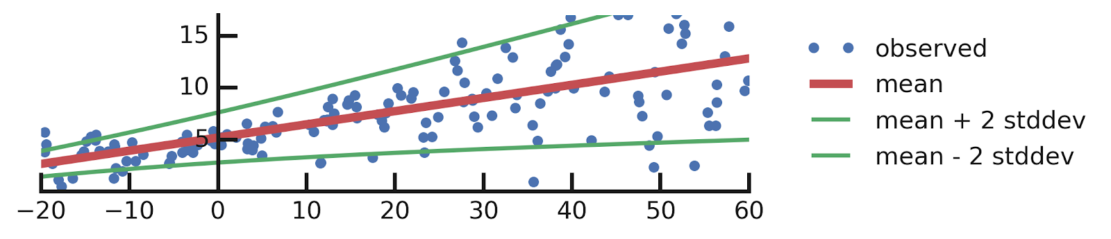
- Aleatoric Uncertainties
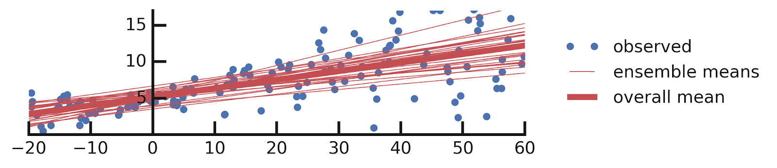
- Epistemic Uncertainties
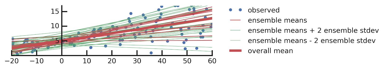
- Epistemic+ Aleatoric Uncertainties
\hat{y} = a x
\hat{y} \sim \mathcal{N}(a x, \sigma^2)
\hat{y} = w x \quad w \sim p(w | \{x_i, y_i\})
\hat{y} \sim \mathcal{N}(w x, \sigma^2) \\ w, \sigma \sim p(w, \sigma | \{x_i, y_i\})
Modeling Aleatoric Uncertainties
A Motivating Example: Image Deconvolution
y = P \ast x + n


Observed y
Unkown x
Ground-based telescope
Hubble Space Telescope

\tilde{x} = f_\theta(y)
-
Step I: Assemble from data or simulations a training set of images $$\mathcal{D} = \{(x_0, y_0), (x_1, y_1), \ldots, (x_N, y_N) \}$$ => the dataset contains hardcoded assumptions about PSF P, noise n, and galaxy morphology x.
- Step II: Train the neural network under a regression loss of the type: $$ \mathcal{L} = \sum_{i=0}^N \parallel x_i - f_\theta(y_i)\parallel^2 $$

y
f_\theta(y)
\mathrm{True } \ x
f_\theta

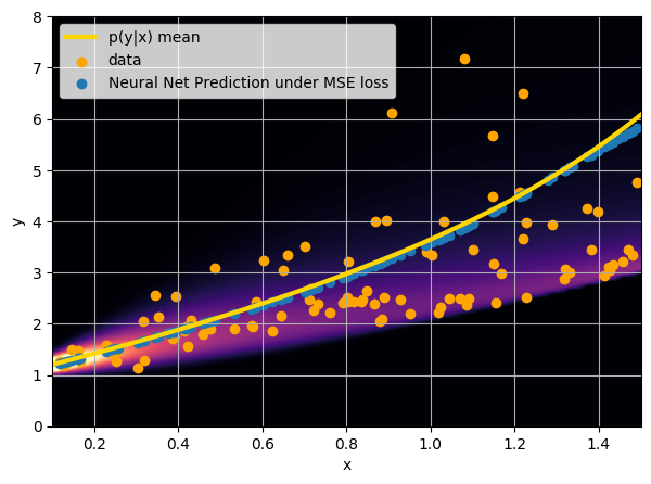
Let's try to understand the neural network output by looking at the loss function
$$ \mathcal{L} = \sum_{(x_i, y_i) \in \mathcal{D}} \parallel x_i - f_\theta(y_i)\parallel^2 \quad \simeq \quad \int \parallel x - f_\theta(y) \parallel^2 \ p(x,y) \ dx dy $$ $$\Longrightarrow \int \left[ \int \parallel x - f_\theta(y) \parallel^2 \ p(x|y) \ dx \right] p(y) dy $$
This is minimized when $$f_{\theta^\star}(y) = \int x \ p(x|y) \ dx $$
i.e. when the network is predicting the mean of p(x|y).
y
\mathrm{True } \ x
p(x|y)
\mathbb{E}_{x \sim p(x|y)}[x]
q_\varphi(\theta= \mathrm{cat} | x) = 0.9
x
credit: Venkatesh Tata
Let's start with binary classification
\theta
=> This means expressing the posterior as a Bernoulli distribution with parameter predicted by a neural network
How do we adjust this parametric distribution to match the true posterior ?
Step 1: We neeed some data
\mathcal{D} = \{ (x_i, \theta_i) \}_{i \in [0, N]}
cat or dog image
label 1 for cat, 0 for dog
(x, \theta) \sim p(x, \theta) = p(\theta) p(x | \theta)
Probability of including cats and dogs in my dataset
Implicit prior
Image search results for cats and dogs
Implicit likelihood
A distance between distributions: the Kullback-Leibler Divergence
D_{KL} (p || q) = \mathbb{E}_{x \sim p(x)} \left[ \log \frac{p(x)}{q(x)} \right]
Step 2: We need a tool to compare distributions
D_{KL} \left( p(x, \theta) || q_\varphi(\theta| x) p(x) \right) = - \mathbb{E}_{p(x,\theta)} \left[ \log \frac{ q_\varphi(\theta | x) p(x) }{ p(x) p(\theta | x) } \right]
= - \mathbb{E}_{p(x, \theta)} \left[ \log q_\varphi(\theta | x) \right] + cst
Minimizing this KL divergence is equivalent to minimizing the negative log likelihood of the model
D_{KL} \left( p(x, \theta) || q_\varphi(\theta | x) p(x) \right) = 0
\\
<=>
\\
q_\varphi(\theta | x) = p(\theta | x)
In our case of binary classification:
\mathbb{E}_{p(x,\theta)}[ - \log q_\varphi(\theta | x)] =\\ \sum_{i=1}^{N} p(1|x_i) \log q_\varphi(1 | x_i) + (1-p(1|x_i)) \log_\varphi(1 | x_i)
We recover the binary cross entropy loss function !
The Probabilistic Deep Learning Recipe
- Express the output of the model as a distribution
- Optimize for the negative log likelihood
- Maybe adjust by a ratio of proposal to prior if the training set is not distributed according to the prior
- Profit!
q_\varphi(\theta | x)
\mathcal{L} = - \log q_\varphi(\theta | x)
q_\varphi(\theta | x) \propto \frac{\tilde{p}(\theta)}{p(\theta)} p(\theta | x)
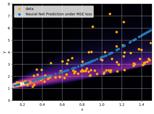
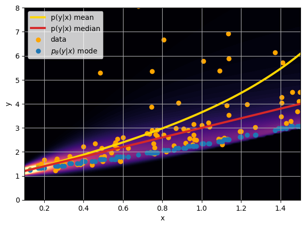
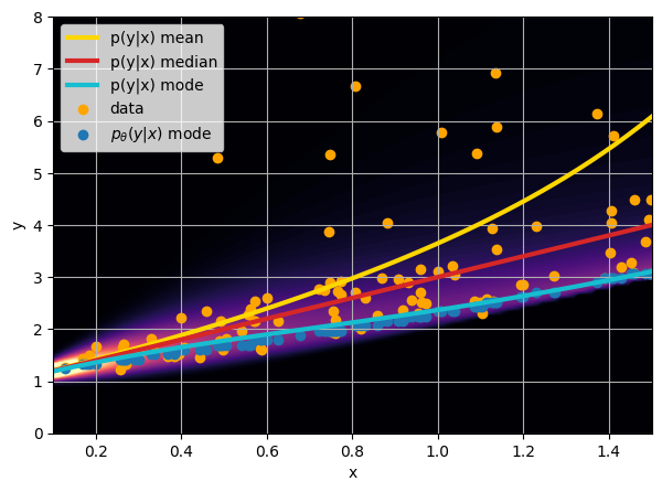
Let us consider a toy regression example
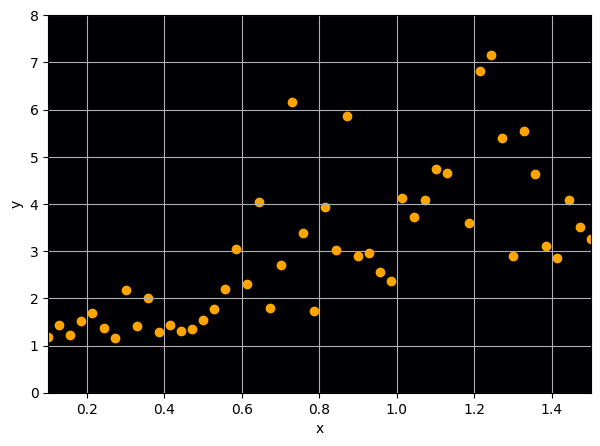
There are intrinsic uncertainties in this problem, at each x there is a full
- Option 1) Train a neural network to learn a function under an MSE loss:
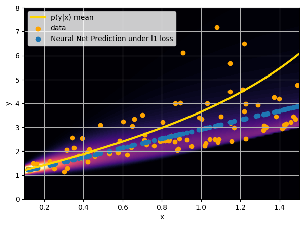
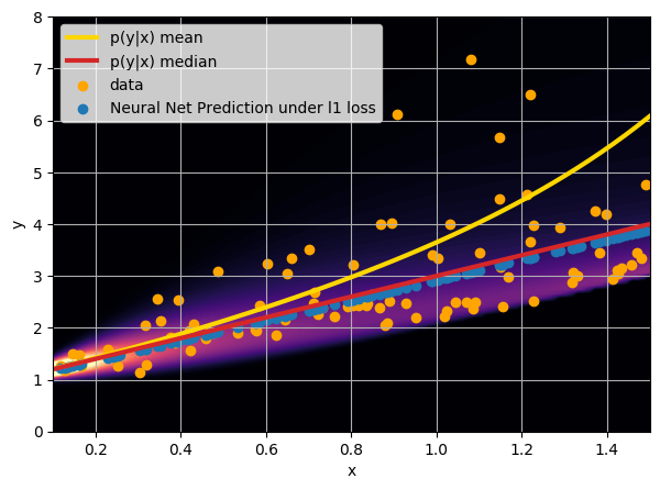
- Option 2) Train a neural network to learn a function under an l1 loss:
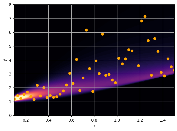
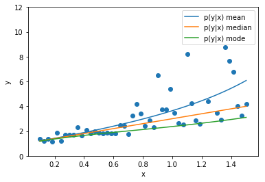
- Option 3) Train a neural network to learn a distribution using a Maximum Likelihood loss
\hat{y} = f_\varphi(x)
\mathcal{L} = \parallel y - f_\varphi(x) \parallel_2^2
p(y | x)
I have a set of data points {x, y} where I observe x and want to predict y.
\hat{y} = f_\varphi(x)
\mathcal{L} = | y - f_\varphi(x) |
p_\varphi(y | x)
\mathcal{L} = - \log p_\varphi(y | x )
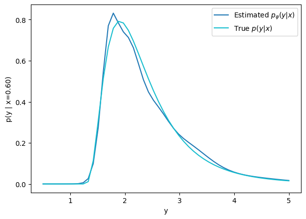
How do we model distributions?
We need a parametric conditional distribution to
compute
- Mixture Density Networks
Bishop 1994
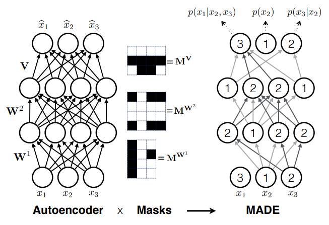
- Autoregressive models
e.g. MADE (Germain et al. 2015)
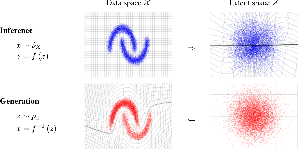
- Normalizing Flows
e.g. MAF (Papamakarios et al. 2017)
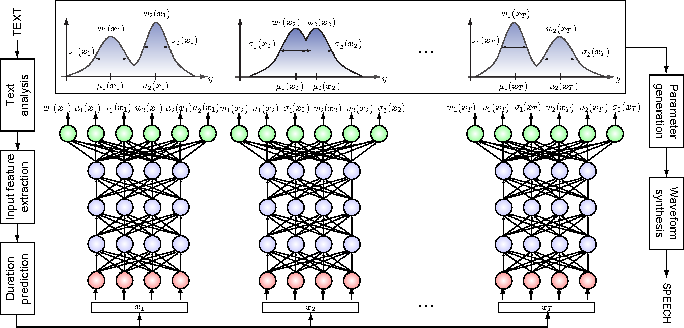
\log p_\varphi(y | x)
p_\varphi(y | x) = \sum_{i=1}^K \pi_i \mathcal{N}( \mu_\varphi(x), \Sigma_\varphi(x))
p_\varphi(y | x) = \Pi_{d=1}^D p_\varphi(y_d | y_1, \ldots, y_{d-1}, x)
p_\varphi(y | x) = p(z = f_\varphi(y, x)) \left| \det \frac{\partial f_\varphi}{\partial z} \right|
How do we do this in practice?
import tensorflow as tf
import tensorflow_probability as tfp
tfd = tfp.distributions

# Build model.
model = tf.keras.Sequential([
  tf.keras.layers.Dense(1+1),
  tfp.layers.IndependentNormal(1),
])

# Define the loss function:
negloglik = lambda x, q: - q.log_prob(x)

# Do inference.
model.compile(optimizer='adam', loss=negloglik)
model.fit(x, y, epochs=500)

# Make predictions.
yhat = model(x_tst)
Let's try it out!
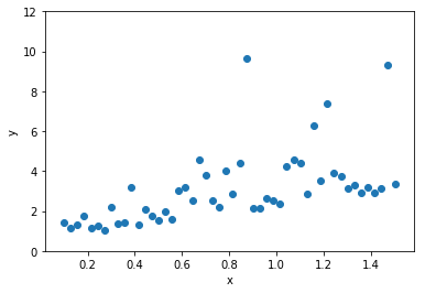
This is our data
Build a regression model for y gvien x
import tensorflow.keras as keras
import tensorflow_probability as tfp

# Number of components in the Gaussian Mixture
num_components = 16

# Shape of the distribution
event_shape = [1]

# Utility function to compute how many parameters this distribution requires

params_size = tfp.layers.MixtureNormal.params_size(num_components, event_shape)

gmm_model = keras.Sequential([
    keras.layers.Dense(units=128, activation='relu', input_shape=(1,)),
    keras.layers.Dense(units=128, activation='tanh'),
    keras.layers.Dense(params_size),
    tfp.layers.MixtureNormal(num_components, event_shape)
])

negloglik = lambda y, q: -q.log_prob(y)

gmm_model.compile(loss=negloglik, optimizer='adam')

gmm_model.fit(x_train.reshape((-1,1)), y_train.reshape((-1,1)),
batch_size=256, epochs=20)A Concrete Example: Estimating Masses of Galaxy Clusters
Try it out at this notebook
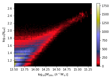
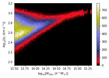
We want to make dynamical mass measurements using information from member galaxy velocity dispersion and about the radial distance distribution (see Ho et al. 2019).
First attempt with an MSE loss
regression_model = keras.Sequential([
    keras.layers.Dense(units=128, activation='relu', input_shape=(14,)),
    keras.layers.Dense(units=128, activation='relu'),
    keras.layers.Dense(units=64, activation='tanh'),
    keras.layers.Dense(units=1)
])

regression_model.compile(loss='mean_squared_error', optimizer='adam')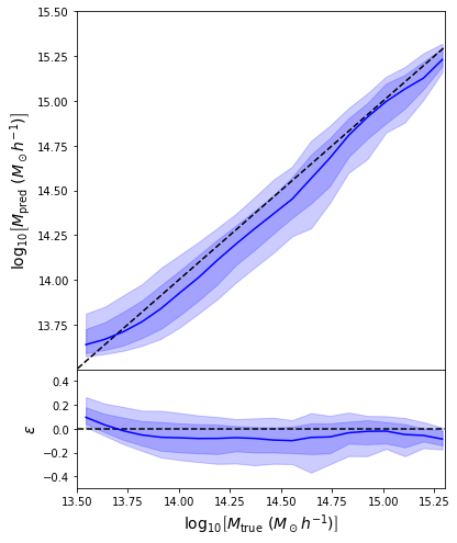
- Simple Dense network using 14 features derived from galaxy positions and velocity information
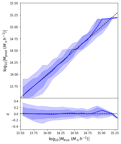
- We see that the predictions are biased compared to the true value of the mass... Not good.
Second attempt: Probabilistic Modeling
num_components = 16
event_shape = [1]

model = keras.Sequential([
    keras.layers.Dense(units=128, activation='relu', input_shape=(14,)),
    keras.layers.Dense(units=128, activation='relu'),
    keras.layers.Dense(units=64, activation='tanh'),
    keras.layers.Dense(tfp.layers.MixtureNormal.params_size(num_components, event_shape)),
    tfp.layers.MixtureNormal(num_components, event_shape)
    ])

negloglik = lambda y, p_y: -p_y.log_prob(y)

model.compile(loss=negloglik, optimizer='adam')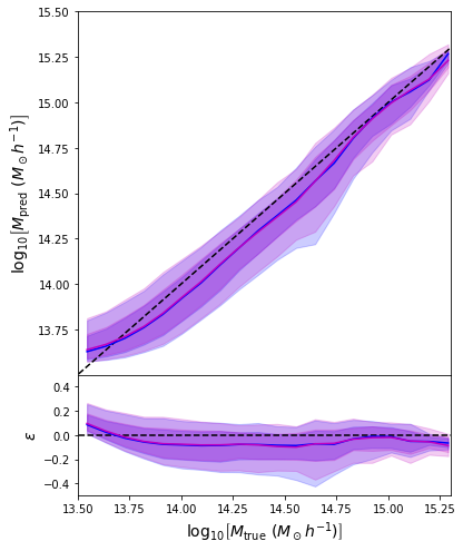
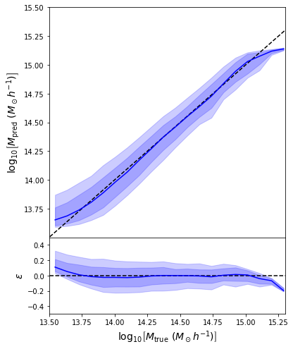
- Same Dense network but now using a Mixture Density output.
- Using the mean of the predicted distribution as our mass estimate: We see the exact same behaviour
What am I doing wrong???
Back to our Dynamical Mass Predictions
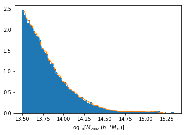
Distribution of masses in our training data

q(M_{200c} | x ) \propto \frac{\tilde{p}(M_{200c})}{p(M_{200c})} p(M_{200c} | x)
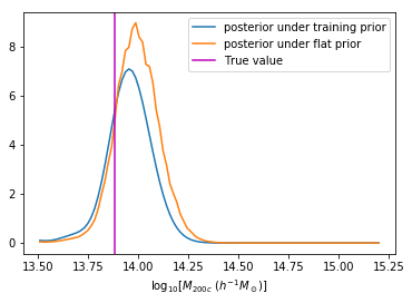
We can reweight the predictions for a desired prior
Last detail, use the mode instead of the mean posterior
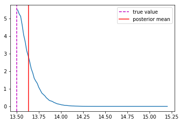
Takeaway Message
- Using a model that outputs distributions instead of scalars is always better!
- It's 2 lines of TensorFlow Probability
- Careful about interpreting these distributions as a Bayesian posterior, the training set acts as an Interim Prior, not necessarily matching your Bayesian prior.
Modeling Epistemic Uncertainties
A Quick reminder
From this excellent tutorial:
- Linear regression
- Aleatoric Uncertainties
- Epistemic Uncertainties
- Epistemic+ Aleatoric Uncertainties
\hat{y} = a x
\hat{y} \sim \mathcal{N}(a x, \sigma^2)
\hat{y} = w x \quad w \sim p(w | \{x_i, y_i\})
\hat{y} \sim \mathcal{N}(w x, \sigma^2) \\ w, \sigma \sim p(w, \sigma | \{x_i, y_i\})
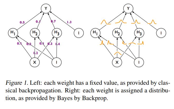
The idea behind Bayesian Neural Networks
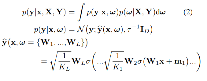
Given a training set D = {X,Y}, the predictions from a Neural Network can be expressed as:
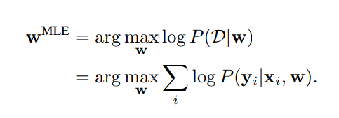
Weight Estimation by Maximum Likelihood
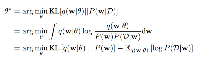
Weight Estimation by Variational Inference
A first approach to BNNs:
Bayes by Backprop (Blundel et al. 2015)
-
Step 1: Assume a variational distribution for the weights of the Neural Network
-
Step 2: Assume a prior distribution for these weights
- Step 3: Learn the parameters of the variational distribution by minimizing the ELBO
q_\theta(w) = \mathcal{N}( \mu_\theta, \Sigma_\theta )
p(w) = \mathcal{N}(0, I)
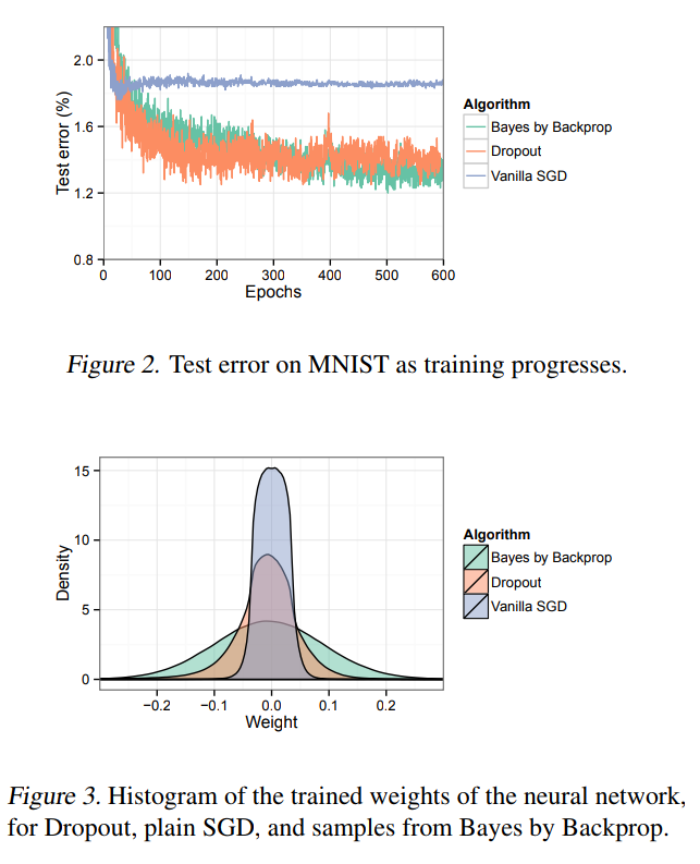
What happens in practice
TensorFlow Probability implementation
A different approach:
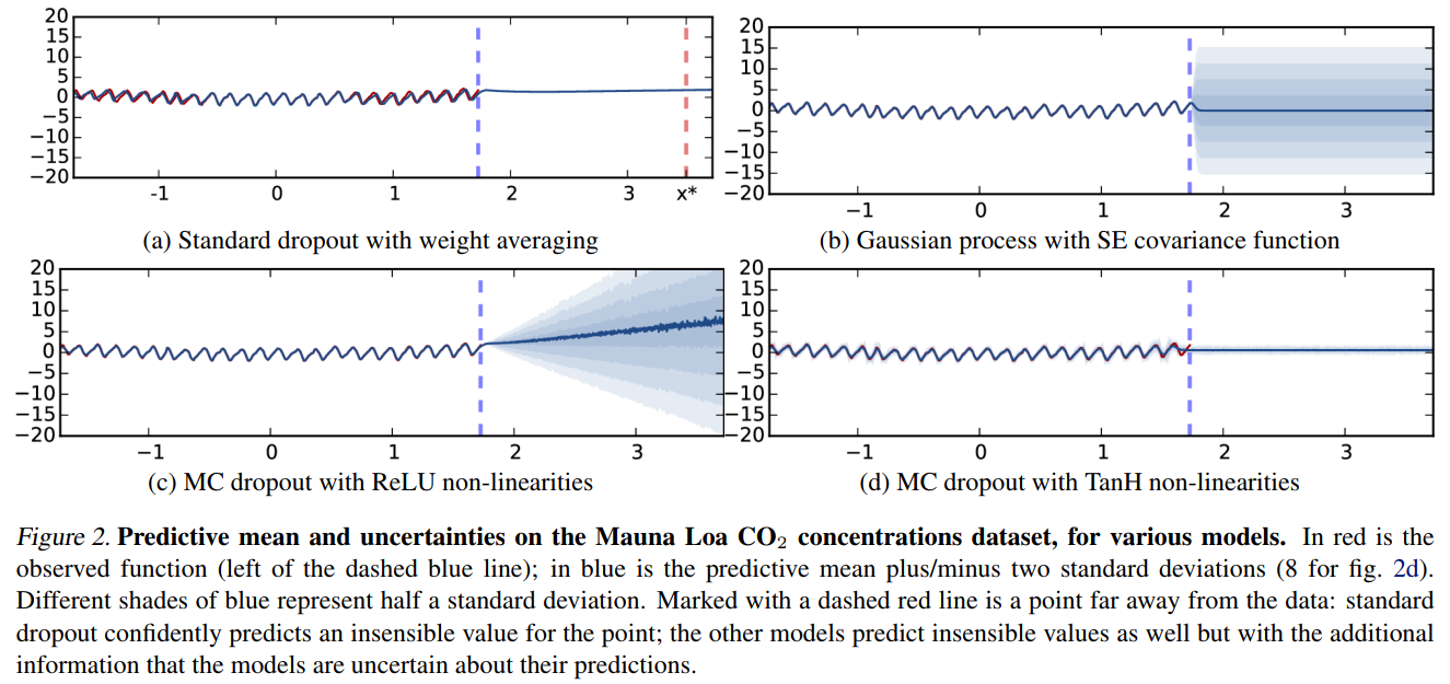
Dropout as a Bayesian Approximation (Gal & Ghahramani, 2015)
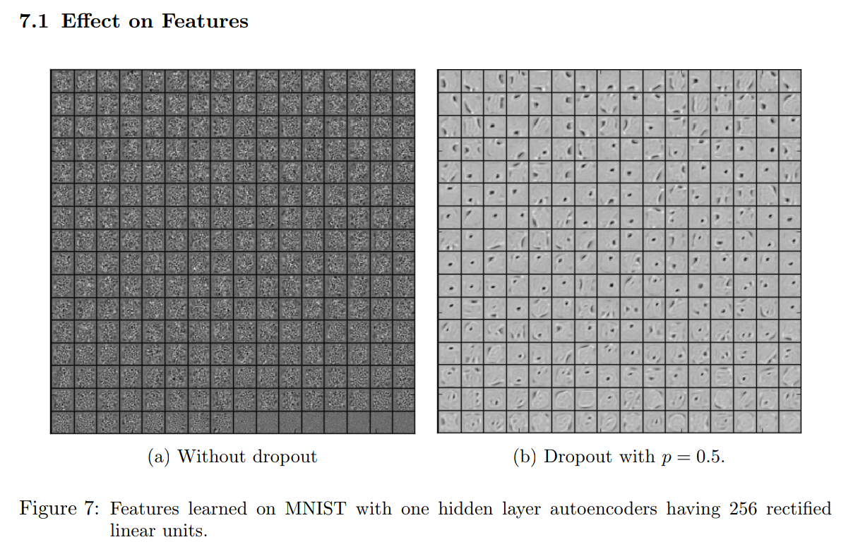
Quick reminder on dropout
Hinton 2012, Srivastava 2014

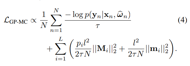
Variational Distribution of Weights under Dropout
-
Step 1: Assume a Variational Distribution for the weights
-
Step 2: Assume a Gaussian prior for the weights, with "length scale" l
- Step 3: Fit the parameters of the variational distribution by optimizing the ELBO

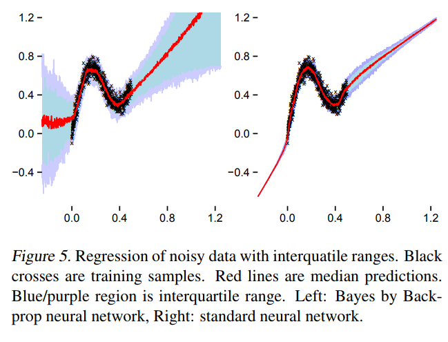
Example
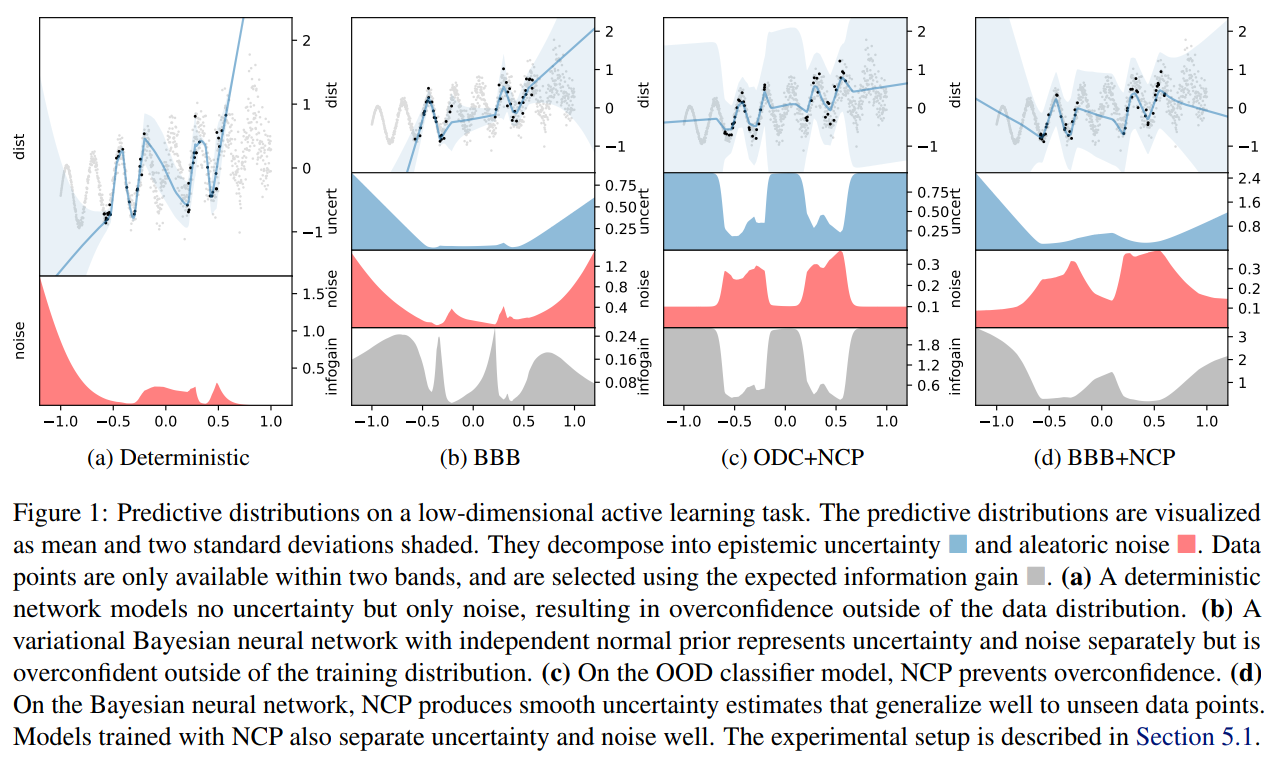
These are not the only methods
- Noise contrastive priors: https://arxiv.org/abs/1807.09289
Takeaway message on Bayesian Neural Networks
- They give a practical way to model epistemic uncertainties, aka unknowns unknows, aka errors on errors
- Be very careful when interpreting their output distributions, they are Bayesian posterior, yes, but under what priors?
- Having access to model uncertainties can be used for active sampling
Putting it all together
Deep Probabilistic Learning
By eiffl
Deep Probabilistic Learning
Probabilistic Learning lecture at Astroinfo 2021


