Probabilistic Learning
in JAX/Flax and TensorFlow Probability

Francois Lanusse @EiffL
+ p(x) =


Our case study
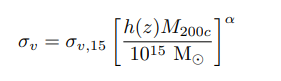
Dynamical Mass Measurement for Galaxy Clusters
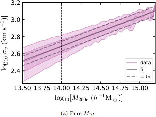
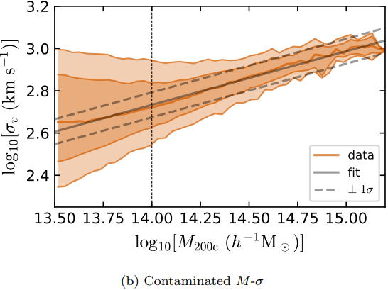
Figures and data from Ho et al. 2019
Our Goal: Train a Neural Network to Estimate Cluster Masses
What we will feed the model:
- Richness
- Velocity Dispersion
- Information about member galaxies:
- radial distribution
- stellar mass distribution
- LOS velocity distribution
Training data from MultiDark Planck 2 N-body simulation (Klypin et al. 2016) with 261287 clusters.
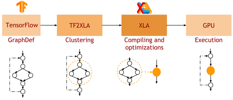
Why JAX?
and what is it?


JAX: NumPy + Autograd + XLA
- JAX uses the NumPy API
=> You can copy/paste existing code, works pretty much out of the box
- JAX is a successor of autograd
=> You can transform any function to get forward or backward automatic derivatives (grad, jacobians, hessians, etc)
- JAX uses XLA as a backend
=> Same framework as used by TensorFlow (supports CPU, GPU, TPU execution)
import jax.numpy as np

m = np.eye(10) # Some matrix

def my_func(x):
  return m.dot(x).sum()

x = np.linspace(0,1,10)
y = my_func(x)
from jax import grad
df_dx = grad(my_func)
y = df_dx(x)
-
Pure functions
=> JAX is designed for functional programming: your code should be built around pure functions (no side effects)- Enables caching functions as XLA expressions
- Enables JAX's extremely powerful concept of composable function transformations
-
Just in Time (jit) Compilation
=> jax.jit() transformation will compile an entire function as XLA, which then runs in one go on GPU.
-
Arbitrary order forward and backward autodiff
=> jax.grad() transformation will apply the d/dx operator to a function f
-
Auto-vectorization
=> jax.vmap() transformation will add a batch dimension to the input/output of any function
def pure_fun(x):
  return 2 * x**2 + 3 * x + 2


def impure_fun_side_effect(x):
  print('I am a side effect')
  return 2 * x**2 + 3 * x + 2


C = 10. # A global variable
def impure_fun_uses_globals(x):
  return 2 * x**2 + 3 * x + C
# Decorator for jitting
@jax.jit
def my_fun(W, x):
return W.dot(x)
# or as an explicit transformation
my_fun_jitted = jax.jit(my_fun)def f(x):
return 2 * x**2 + 3 *x + 2
df_dx = jax.grad(f)
jac = jax.jacobian(f)
hess = jax.hessian(f)
# As decorator
@jax.vmap
def f(x):
  return 2 * x**2 + 3 *x + 2

# Can be composed
df_dx = jax.jit(jax.vmap(jax.grad(f)))
Writing a Neural Network in JAX/Flax
import flax.linen as nn
import optax

class MLP(nn.Module):
  @nn.compact
  def __call__(self, x):
    x = nn.relu(nn.Dense(128)(x))
    x = nn.relu(nn.Dense(128)(x))
    x = nn.Dense(1)(x)
    return x
# Instantiate the Neural Network
model = MLP()
# Initialize the parameters
params = model.init(jax.random.PRNGKey(0), x)
prediction = model.apply(params, x)
# Instantiate Optimizer
tx = optax.adam(learning_rate=0.001)
opt_state = tx.init(params)
# Define loss function
def loss_fn(params, x, y):
  mse = model.apply(params, x) -y)**2
  return jnp.mean(mse)
# Compute gradients
grads = jax.grad(loss_fn)(params, x, y)
# Update parameters
updates, opt_state = tx.update(grads, opt_state)
params = optax.apply_updates(params, updates)- Model Definition: Subclass the flax.linen.Module base class. Only need to define the __call__() method.
-
Using the Model: the model instance provides 2 important methods:
- init(seed, x): Returns initial parameters of the NN
- apply(params, x): Pure function to apply the NN
- Training the Model: Use jax.grad to compute gradients and Optax optimizers to update parameters
Now You Try it!
We will be using this notebook
Your goal: Building a regression model with a Mean Squared Error loss in JAX/Flax
def loss_fn(params, x, y):
  mse = (model.apply(params, x) - y)**2
  return jnp.mean(mse)
Raise your hand when you reach the cluster mass prediction plot
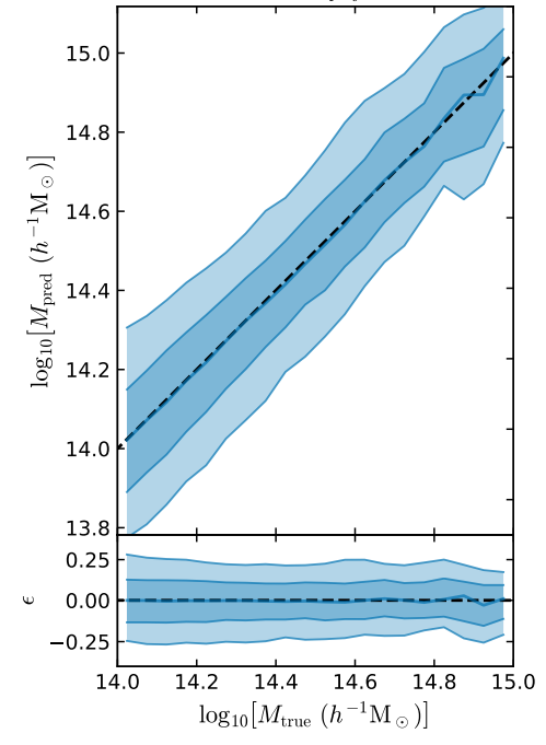
First attempt with an MSE loss
class MLP(nn.Module):
  @nn.compact
  def __call__(self, x):
    x = nn.relu(nn.Dense(128)(x))
    x = nn.relu(nn.Dense(128)(x))
    x = nn.tanh(nn.Dense(64)(x))
    x = nn.Dense(1)(x)
    return x

def loss_fn(params, x, y):
  prediction = model.apply(params, x)
  return jnp.mean( (prediction - y)**2 )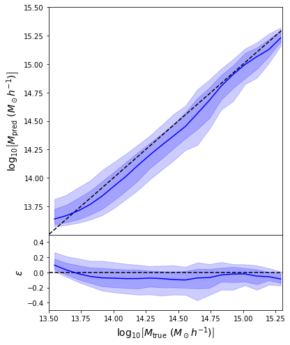
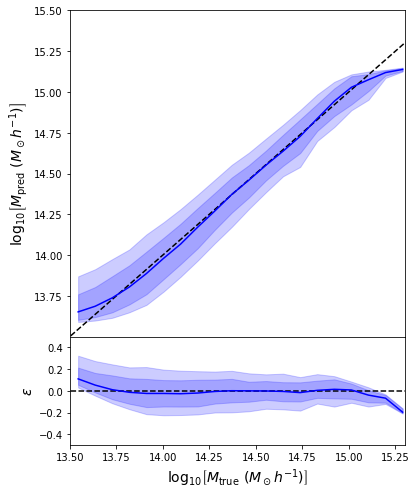
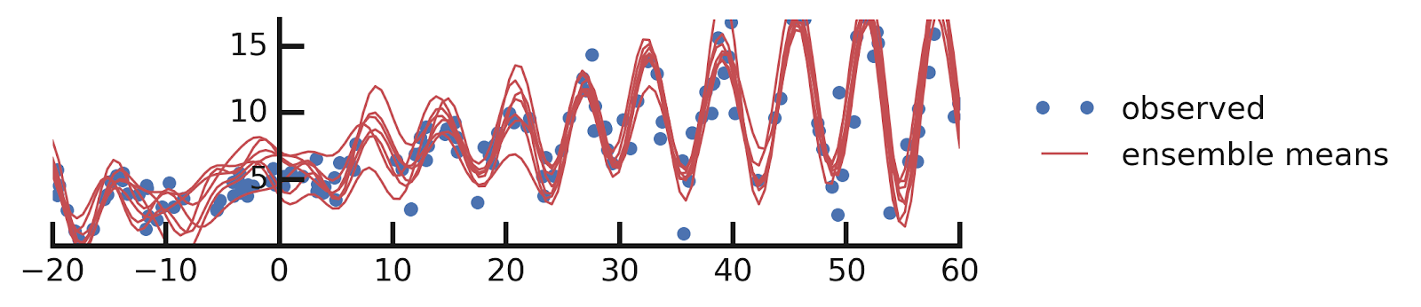
- Simple Dense network using 14 features derived from galaxy positions and velocity information
- We see that the predictions are biased compared to the true value of the mass... Not good.
What is going on???

We need a new tool to go probabilistic
import jax
import jax.numpy as jnp
from tensorflow_probability.substrates import jax as tfp
tfd = tfp.distributions

### Create a mixture of two scalar Gaussians:
gm = tfd.MixtureSameFamily(
  mixture_distribution=tfd.Categorical(
                 probs=[0.3, 0.7]),
  components_distribution=tfd.Normal(
                 loc=[-1., 1],
                 scale=[0.1, 0.5]))

# Evaluate probability
gm.log_prob(1.0)
Let's build a Conditional Density Estimator with TFP
class MDN(nn.Module):
  num_components: int

  @nn.compact
  def __call__(self, x):
    x = nn.relu(nn.Dense(128)(x))
    x = nn.relu(nn.Dense(128)(x))
    x = nn.tanh(nn.Dense(64)(x))

    # Instead of regressing directly the value of the mass, the network
    # will now try to estimate the parameters of a mass distribution.
    categorical_logits = nn.Dense(self.num_components)(x)
    loc = nn.Dense(self.num_components)(x)
    scale = 1e-3 + nn.softplus(nn.Dense(self.num_components)(x))

    dist =tfd.MixtureSameFamily(
        mixture_distribution=tfd.Categorical(logits=categorical_logits),
        components_distribution=tfd.Normal(loc=loc, scale=scale))

    # To make it understand the batch dimension
    dist =  tfd.Independent(dist)

    # Returns a distribution !
    return dist
Now you try it!
Your goal: Implement a Mixture Density Network in JAX/Flax/TFP, and use it to get unbiased mass estimates.
When everyone is done, we will discuss the results.
def loss_fn(params, x, y):
  q = model.apply(params, x)
  return jnp.mean( - q.log_prob(y[:,0]) )
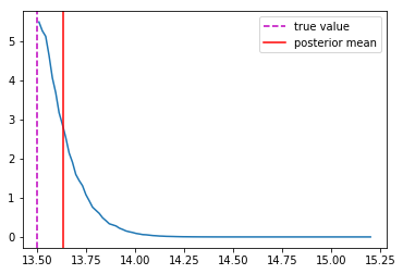
Second attempt: Probabilistic Modeling
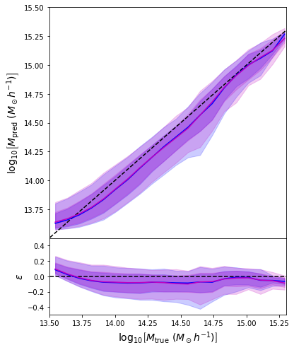
- Same Dense network but now using a Mixture Density output.
- Using the mean of the predicted distribution as our mass estimate: We see the exact same behaviour
What am I doing wrong???
Accounting for Implicit Prior
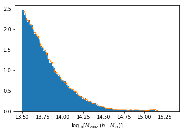
Distribution of masses in our training data

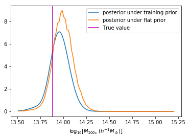
q(M_{200c} | x ) \propto \frac{\tilde{p}(M_{200c})}{p(M_{200c})} p(M_{200c} | x)
We can reweight the predictions for a desired prior
Last detail, use the mode instead of the mean posterior
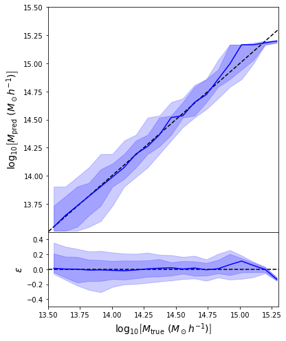
Takeaway Message
- Using a model that outputs distributions instead of scalars is always better!
- It's 2 lines of TensorFlow Probability
- Careful about interpreting these distributions as a Bayesian posterior, the training set acts as an Interim Prior, not necessarily matching your Bayesian prior.
=> Connection with proper Simulation Based Inference by Neural Density Estimation
A brief Mention of How to Model Epistemic Uncertainties
A Quick reminder
From this excellent tutorial:
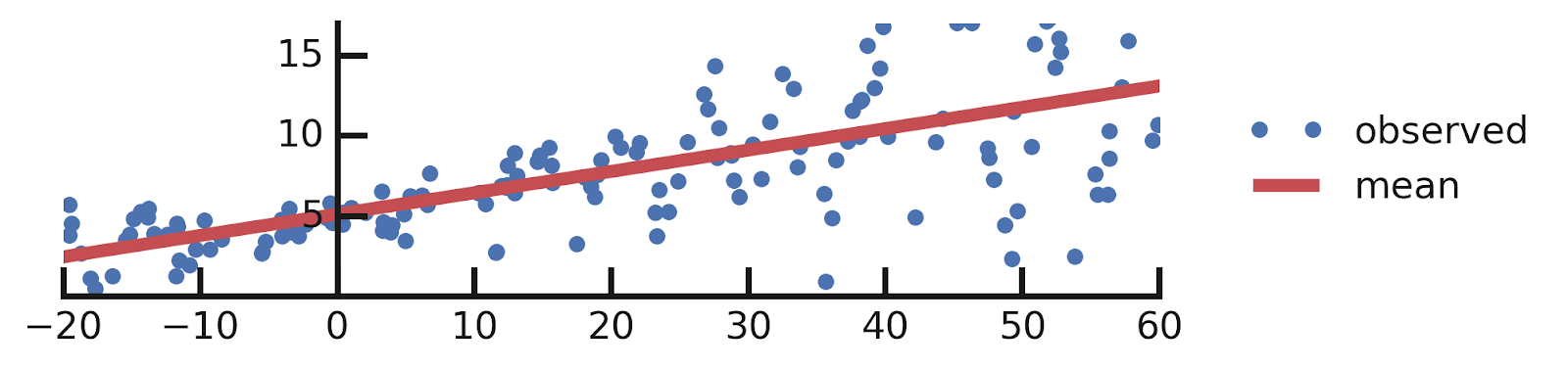
- Linear regression
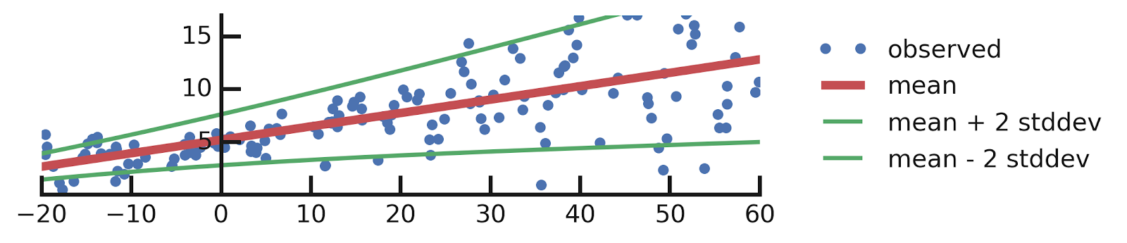
- Aleatoric Uncertainties
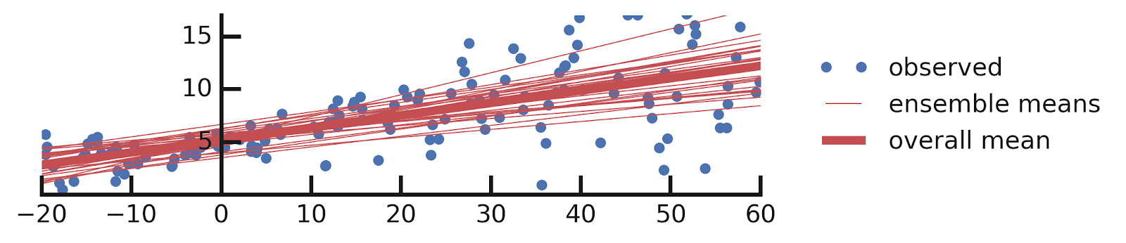
- Epistemic Uncertainties
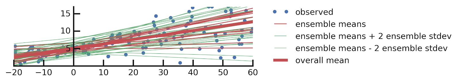
- Epistemic+ Aleatoric Uncertainties
\hat{y} = a x
\hat{y} \sim \mathcal{N}(a x, \sigma^2)
\hat{y} = w x \quad w \sim p(w | \{x_i, y_i\})
\hat{y} \sim \mathcal{N}(w x, \sigma^2) \\ w, \sigma \sim p(w, \sigma | \{x_i, y_i\})
The idea behind Bayesian Neural Networks
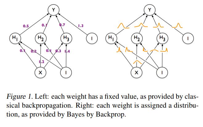
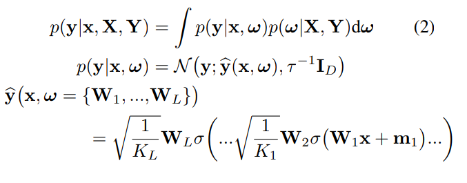
Given a training set D = {X,Y}, the predictions from a Neural Network can be expressed as:
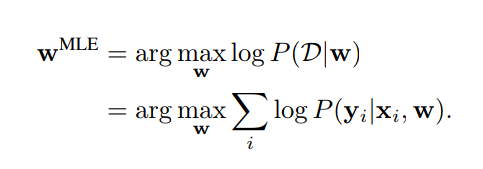
Weight Estimation by Maximum Likelihood
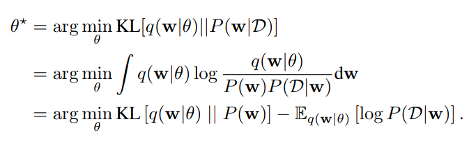
Weight Estimation by Variational Inference
A first approach to BNNs:
Bayes by Backprop (Blundel et al. 2015)
-
Step 1: Assume a variational distribution for the weights of the Neural Network
-
Step 2: Assume a prior distribution for these weights
- Step 3: Learn the parameters of the variational distribution by minimizing the ELBO
q_\theta(w) = \mathcal{N}( \mu_\theta, \Sigma_\theta )
p(w) = \mathcal{N}(0, I)
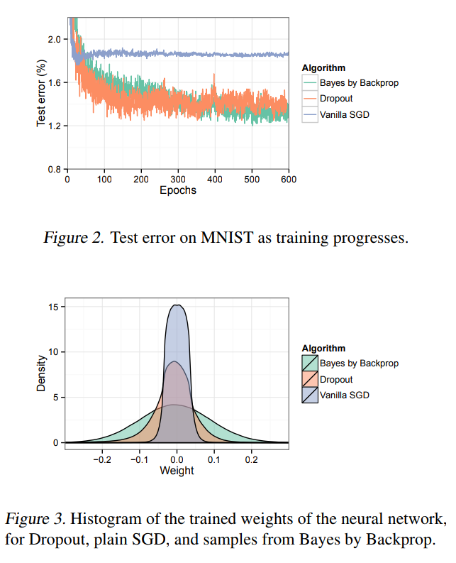
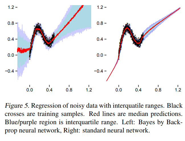
What happens in practice
TensorFlow Probability implementation
A different approach:
Dropout as a Bayesian Approximation (Gal & Ghahramani, 2015)
Quick reminder on dropout
Hinton 2012, Srivastava 2014

Variational Distribution of Weights under Dropout
-
Step 1: Assume a Variational Distribution for the weights
-
Step 2: Assume a Gaussian prior for the weights, with "length scale" l
- Step 3: Fit the parameters of the variational distribution by optimizing the ELBO

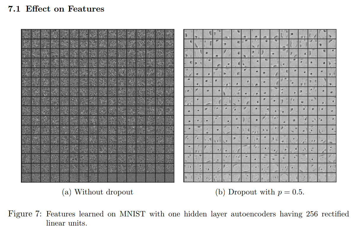
Example
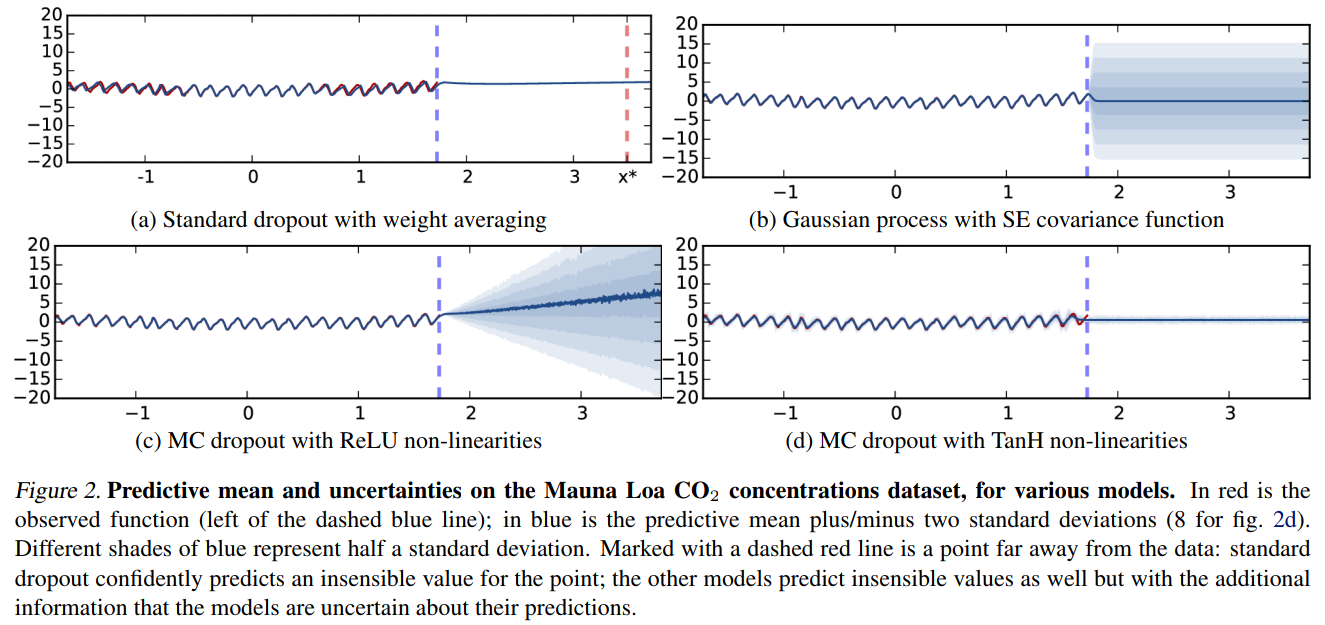
These are not the only methods
- Noise contrastive priors: https://arxiv.org/abs/1807.09289
Takeaway message on Bayesian Neural Networks
- They give a practical way to model epistemic uncertainties, aka unknowns unknows, aka errors on errors
- Be very careful when interpreting their output distributions, they are Bayesian posterior, yes, but under what priors?
- Having access to model uncertainties can be used for active sampling
Solution Notebook
Bonus Notebook Implementing a Normalizing Flow
Introduction to Probabilistic Learning in JAX
By eiffl
Introduction to Probabilistic Learning in JAX
Probabilistic Learning lecture at Kavli IPMU, April 2023


