Simulation-Based Inference for Cosmology - Hands On

Ecole de Physique des Houches

JULY 2025

François Lanusse

Université Paris-Saclay, Université Paris Cité, CEA, CNRS, AIM

https://slides.com/eiffl/sbi

Why JAX?

and what is it?

Credit

JAX: NumPy + Autograd + XLA

JAX uses the NumPy API
=> You can copy/paste existing code, works pretty much out of the box
JAX is a successor of autograd
=> You can transform any function to get forward or backward automatic derivatives (grad, jacobians, hessians, etc)
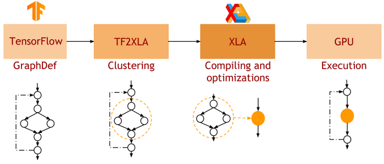
JAX uses XLA as a backend
=> Same framework as used by TensorFlow (supports CPU, GPU, TPU execution)

import jax.numpy as np

m = np.eye(10) # Some matrix

def my_func(x):
  return m.dot(x).sum() 

x = np.linspace(0,1,10)
y = my_func(x)

from jax import grad

df_dx = grad(my_func)
 
y = df_dx(x)

Pure functions
=> JAX is designed for functional programming: your code should be built around pure functions (no side effects)
- Enables caching functions as XLA expressions
- Enables JAX's extremely powerful concept of composable function transformations
Just in Time (jit) Compilation
=> jax.jit() transformation will compile an entire function as XLA, which then runs in one go on GPU.
Arbitrary order forward and backward autodiff
=> jax.grad() transformation will apply the d/dx operator to a function f
Auto-vectorization
=> jax.vmap() transformation will add a batch dimension to the input/output of any function

def pure_fun(x):
  return 2 * x**2 + 3 * x + 2


def impure_fun_side_effect(x):
  print('I am a side effect')
  return 2 * x**2 + 3 * x + 2


C = 10. # A global variable
def impure_fun_uses_globals(x):
  return 2 * x**2 + 3 * x + C

# Decorator for jitting
@jax.jit
def my_fun(W, x):
  return W.dot(x)

# or as an explicit transformation
my_fun_jitted = jax.jit(my_fun)

def f(x):
  return 2 * x**2 + 3 *x + 2

df_dx = jax.grad(f)   
jac = jax.jacobian(f)
hess = jax.hessian(f)

# As decorator
@jax.vmap
def f(x):
  return 2 * x**2 + 3 *x + 2

# Can be composed
df_dx = jax.jit(jax.vmap(jax.grad(f)))

Writing a Neural Network in JAX/Flax

import flax.linen as nn
import optax

class MLP(nn.Module):
  @nn.compact
  def __call__(self, x):
    x = nn.relu(nn.Dense(128)(x))
    x = nn.relu(nn.Dense(128)(x))
    x = nn.Dense(1)(x)
    return x
# Instantiate the Neural Network  
model = MLP()
# Initialize the parameters
params = model.init(jax.random.PRNGKey(0), x)
prediction = model.apply(params, x)
# Instantiate Optimizer
tx = optax.adam(learning_rate=0.001)
opt_state = tx.init(params)
# Define loss function
def loss_fn(params, x, y):
  mse = model.apply(params, x) -y)**2
  return jnp.mean(mse)
# Compute gradients
grads = jax.grad(loss_fn)(params, x, y)
# Update parameters
updates, opt_state = tx.update(grads, opt_state)
params = optax.apply_updates(params, updates)

Model Definition: Subclass the flax.linen.Module base class. Only need to define the __call__() method.
Using the Model: the model instance provides 2 important methods:
- init(seed, x): Returns initial parameters of the NN
- apply(params, x): Pure function to apply the NN
Training the Model: Use jax.grad to compute gradients and Optax optimizers to update parameters