


Erik Jansson
WASP and KAW postdoctoral fellow in the Cambridge Image Analysis Group and CRA at Wolfson College.
Bolin, D., Kirchner, K., Kovács, M., Numerical solution of fractional elliptic stochastic PDEs with spatial white noise, IMA J. Numer. Anal., 40(2):1051–1073, 2020
Dziuk, G., and Elliott, C. M., Finite element methods for surface PDEs. Acta Num., 22:289–396, 2013.
Lang A., Pereira, M., Galerkin–Chebyshev approximation of Gaussian random fields on compact Riemannian manifolds (preprint)
Whittle, P., Stochastic processes in several dimensions. Bull. Inst. Int. Stat., 40:974–994, 1963.
The SPDE view: GRFs are solutions to elliptic stochastic partial differential equations on manifolds:
In this talk: Manifolds = compact, boundary–less 2D embedded surfaces in \(\mathbb{R}^3\)
Elliptic differential operator
White noise
Two questions:
Computation
Statistics
The SPDE view: GRFs are solutions to elliptic stochastic partial differential equations on manifolds:
In this talk: Manifolds = compact, boundary–less 2D embedded surfaces in \(\mathbb{R}^3\)
Elliptic differential operator
White noise
Two questions:
Computation
Statistics
The SPDE view: GRFs are solutions to elliptic stochastic partial differential equations on manifolds:
In this talk: Manifolds = compact, boundary–less 2D embedded surfaces in \(\mathbb{R}^3\)
Elliptic differential operator
White noise
Two questions:
Sampling
Statistics
On surfaces!
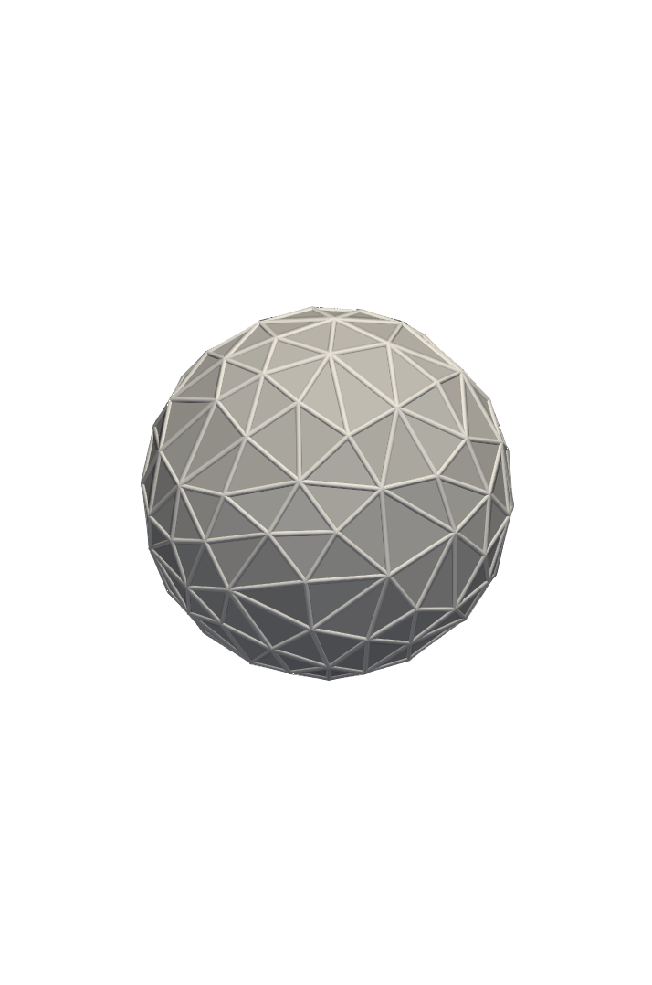
Step 1: Triangulate the surface
Step 2: FEM space \(S_h \subset H^1(\mathcal{M}_h)\) of p.w., continuous, linear functions
Problem 1: Approximate solutions live on \(\mathcal{M}_h\), not \(\mathcal{M}\)!
Step 3: Key tool in surface finite elements: the lift
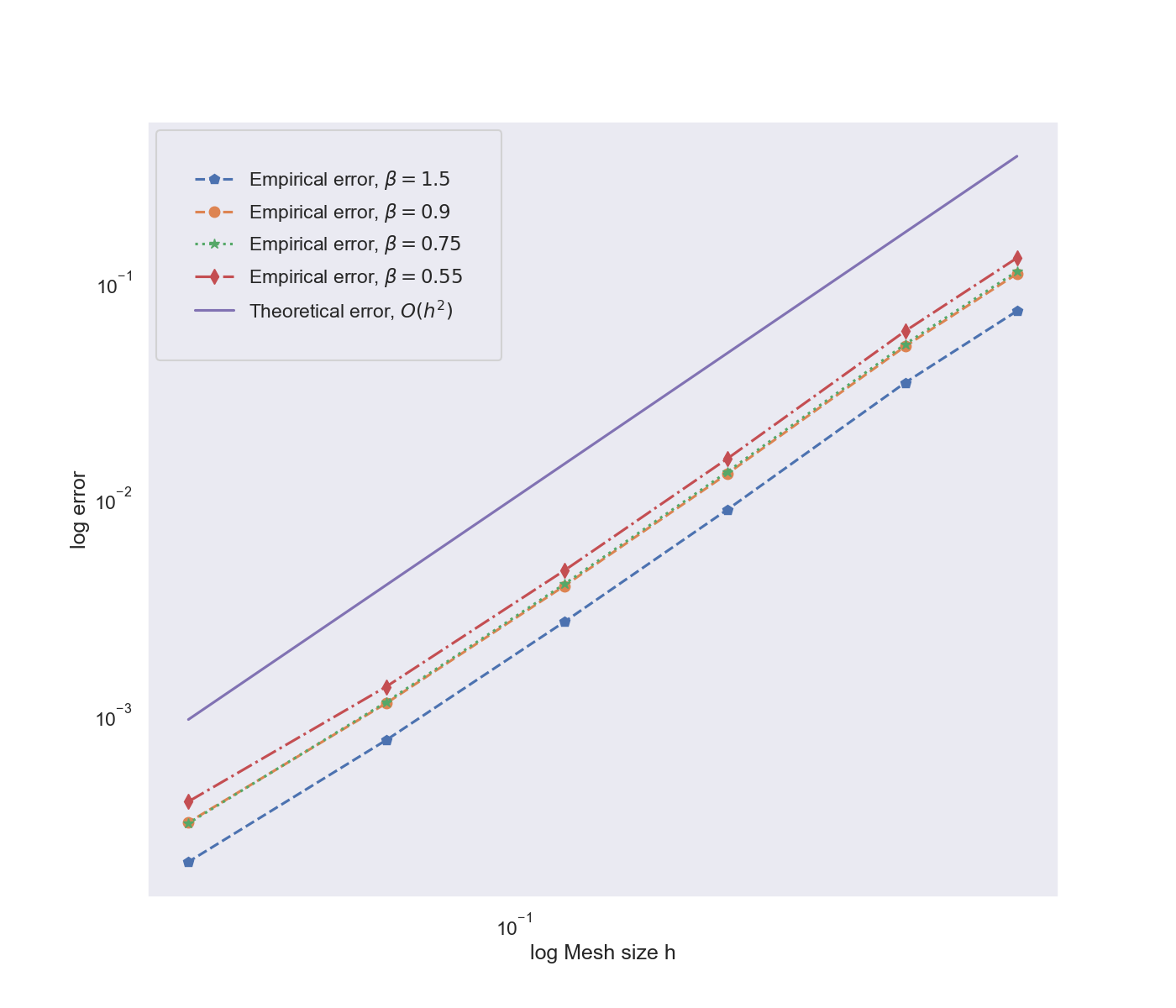
Takeway: FEM error similar to flat case, up to a "geometry error" term
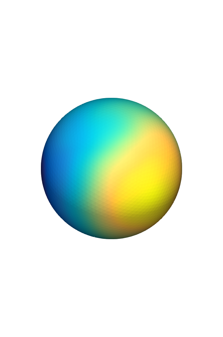
\(\left(\kappa^2-\Delta_{\mathbb{S}^2}\right)^\beta u=\mathcal{W}\), \(\beta>1/2, \kappa \neq 0\)
Question: What to do with fractional operator?
Dunford–Taylor integral representation:
\(\left(\kappa^2-\Delta_{\mathbb{S}^2}\right)^\beta u=\mathcal{W}\), \(\beta>1/2, \kappa \neq 0\)
Question: What to do with noise?
Computable by standard SFEM!
Question: What to do with fractional operator?
Dunford–Taylor integral sinc quadrature:
In E.J, Kovács, M & Lang, A, (2022) strong error bounds are proved.
Problem: How to approximate noise?
Solution: Different approach...
\((\lambda_i,e_i)\) are eigenpairs of \(\mathcal{L}\)
Use power spectral density \(\gamma : \mathbb{R}_+\rightarrow \mathbb{R} \)
Random weights \((W_i : i\in\mathbb{N})\) are Gaussian
Problem: Eigenfunctions are not known.
Solution (?): Approximation with SFEM basis functions
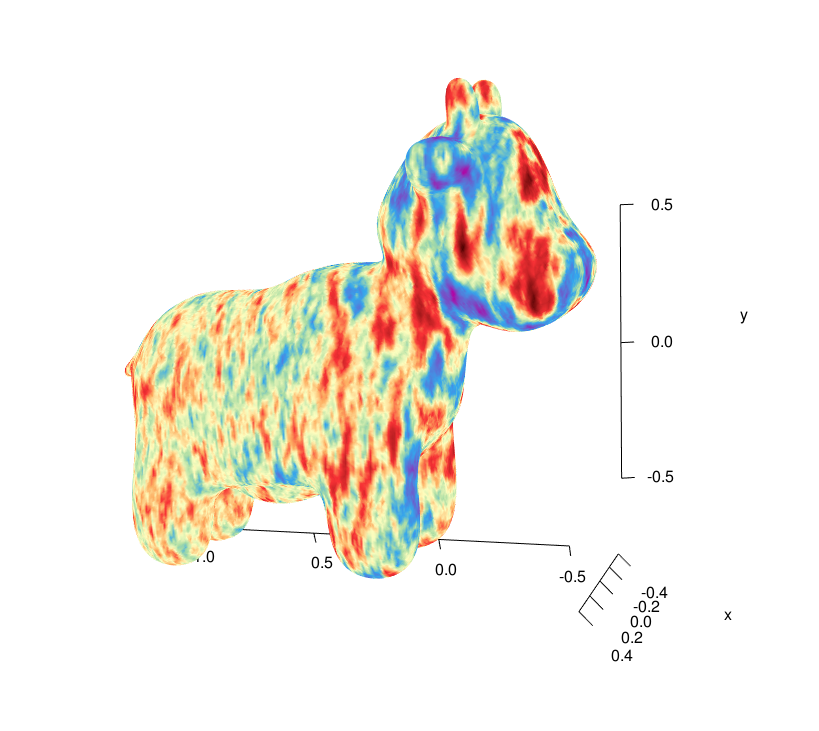
c(x):
small
large
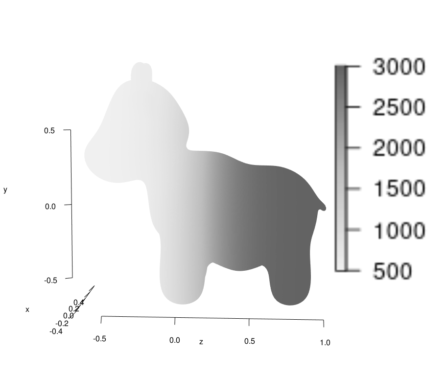
A(x):
Pullback of \(\R^3\) metric
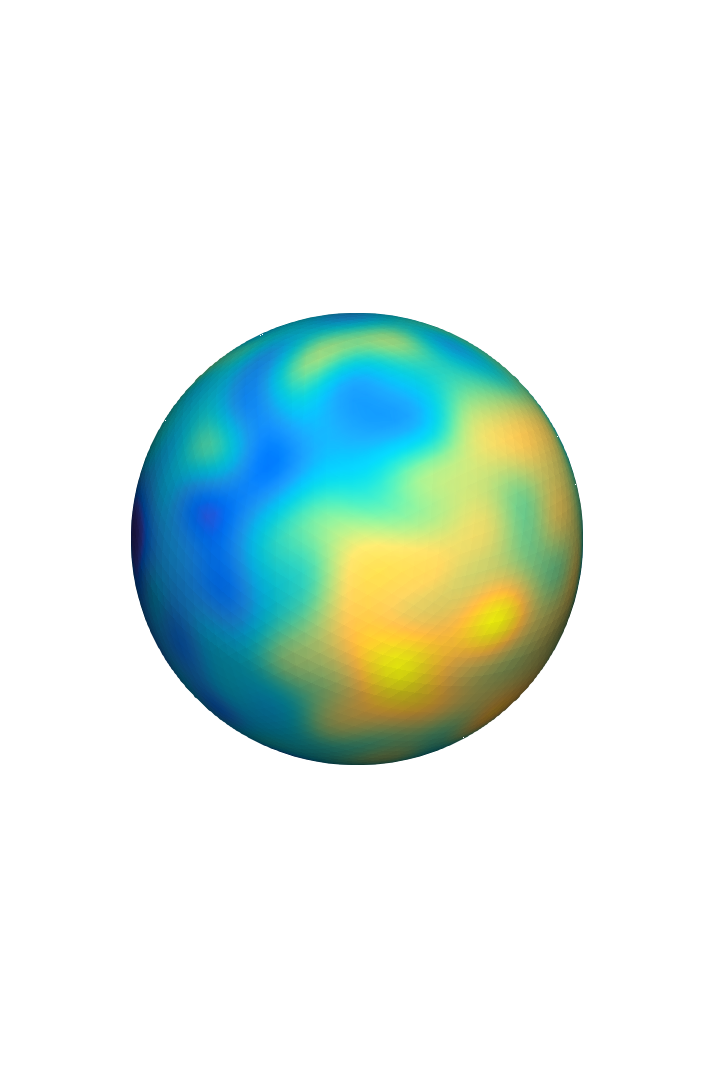
Inverse correlation length: small values, bigger spots.
Smaller correlation length along \(z\)-axis, elongation in that direction!
By Erik Jansson


