

federica bianco PRO
astro | data science | data for good
dr.federica bianco | fbb.space | fedhere | fedhere
Convolutional Neural networks
Neural Networks
mean square error
mean absolute error
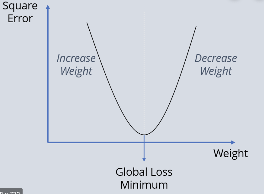
How do we fit a model to data?
minimize loss function
Gradient descent
.
.
.
Any linear model
.
.
.
perceptron or
shallow NN
input layer
hidden layer
output layer
.
.
.
Any linear model
y : prediction
ytrue : target
Error: e.g.
intercept
slope
L2
x
features
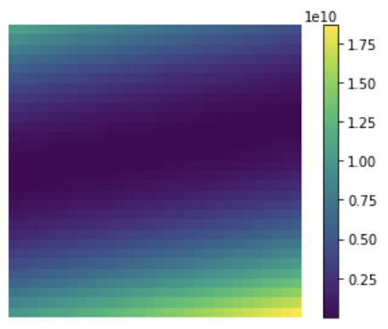
Find the best parameters by finding the minimum of the L2 hyperplane
.
.
.
Any linear model
y : prediction
ytrue : target
Error: e.g.
intercept
slope
L2
Find the best parameters by finding the minimum of the L2 hyperplane
x
.
.
.
Any linear model
y : prediction
ytrue : target
Error: e.g.
intercept
slope
L2
Find the best parameters by finding the minimum of the L2 hyperplane
at every step look around and choose the best direction
global minimum
x
initial
guess
.
intercept
slope
L2
global minimum
x
How do I know in which direction to go?
find the direction where L2 decreases by taking the gradient of the loss function
w respect to the parameters (a,b)
global minimum
L2
initial
guess
.
Find the best parameters by finding the minimum of the L2 hyperplane
at every step look around and choose the best direction
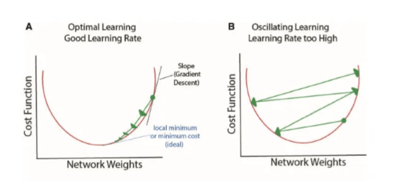
Gradient Descent
Used to optimize parameters of a function fit to data
0. Choose a learning rate hyperparameter α
{
Gradient Descent
Used to optimize parameters of a function fit to data
0. Choose a learning rate hyperparameter α
{
parameter
function f
Find the best parameters by finding the minimum of the L2 hyperplane
at every step look around and choose the best direction
How do I know in which direction to go?
find the direction where L2 decreases by taking the gradient of the loss function
w respect to the parameters (a,b)
global minimum
L2
Gradient Descent
Used to optimize parameters of a function fit to data
def gradDesc(m, b, x, y, alpha, ax=None):
    N = len(x)
    #partial derivative: -2x(y - (mx + b)), -2(y - (mx + b))
    f_m = (-2 * x * (y - (m * x + b))).sum()
    f_b = (-2 * (y - (m * x + b))).sum()
    # We subtract because the derivatives point in direction of steepest ascent
    m -= f_m / float(N) * alpha
    b -= f_b / float(N) * alpha
    return m, b

#initial setup
m_new, b_new = 11, 11

#hyperparmeters
epsilon = 1  #convergence threshold
alpha = 0.0005 #learning rate

print (loss(m, b, x, y))
while  loss(m_new, b_new, x, y) > epsilon:
    #time.sleep(1)
    m_old, b_old = m_new, b_new
    print (loss(m_new, b_new, x, y))
    m_new, b_new = gradDesc(m_old, b_old, x, y, alpha, ax=ax)
Perceptrons are linear classifiers: makes its predictions based on a linear predictor function
combining a set of weights (=parameters) with the feature vector.
.
.
.
output
activation function
weights
bias
output
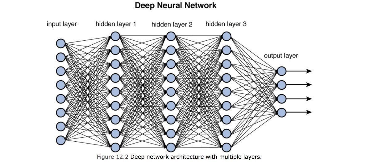
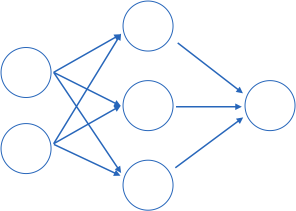
Fully connected: all nodes go to all nodes of the next layer.
input layer
hidden layer
output layer
1970: multilayer perceptron architecture
output
Fully connected: all nodes go to all nodes of the next layer.
layer of perceptrons
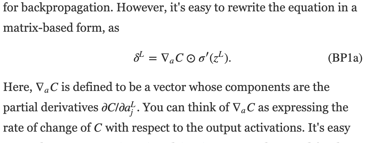
Back
Propagation
how does linear descent look when you have a whole network structure with hundreds of weights and biases to optimize??
.
.
.
output
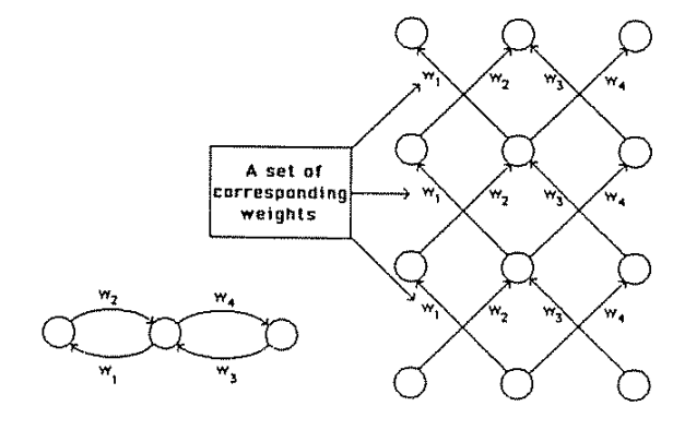
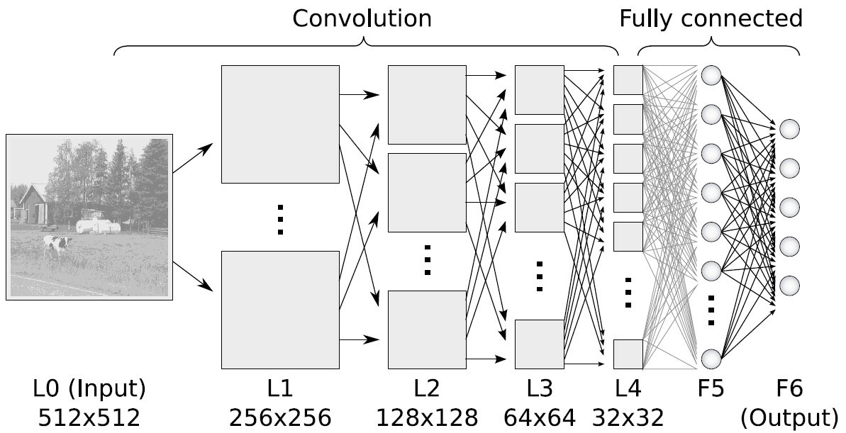
Seminal paper
Y. LeCun 1998
W4
Training models with this many parameters requires a lot of care:
- defining the metric
- choose optimization schemes
- training/validation/testing sets
Small changes in the parameters leads to small changes in the output for the right activation functions.
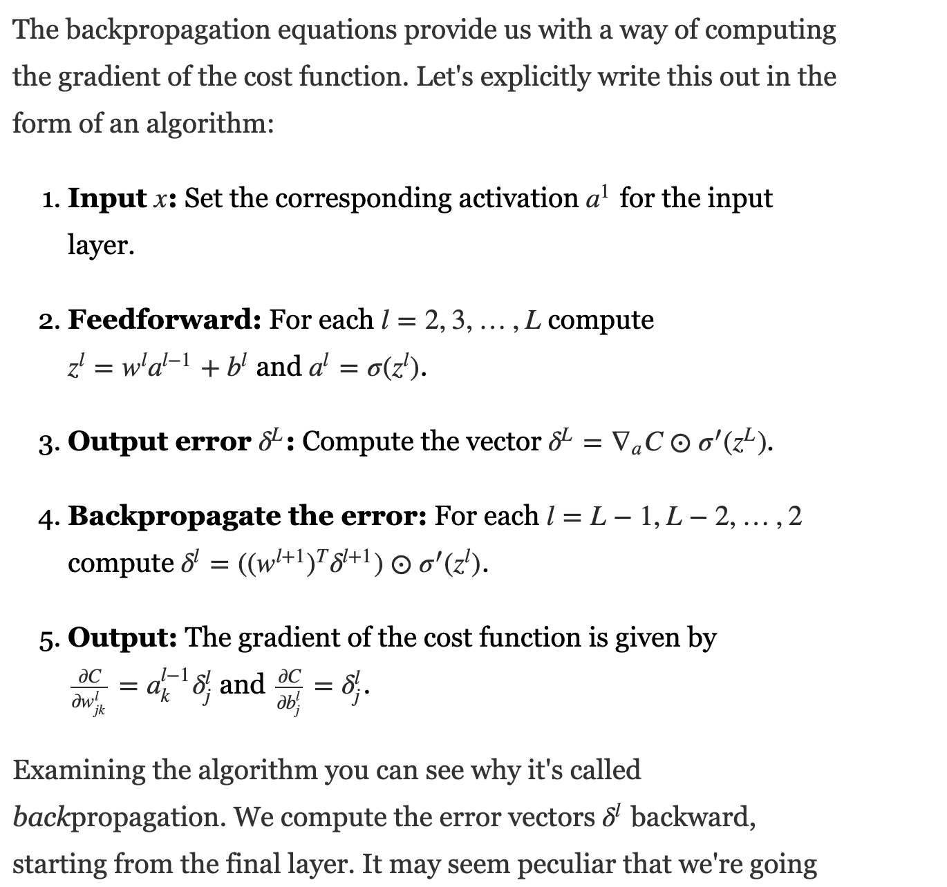
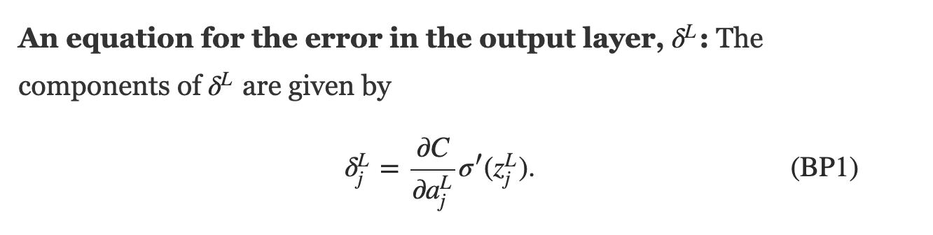
Training a DNN
feed data forward through network and calculate cost metric
for each layer, calculate effect of small changes on next layer
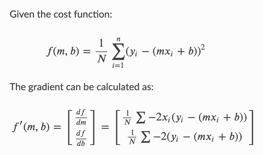
define a cost function, e.g.
how does linear descent look when you have a whole network structure with hundreds of weights and biases to optimize??
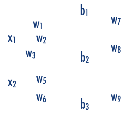
think of applying just gradient to a function of a function of a function... use:
1) partial derivatives, 2) chain rule
define a cost function, e.g.
Training a DNN
Training a DNN
Exploding Gradient
the gradients of the network's loss with respect to the parameters (weights) become excessively large.
The "explosion" of the gradient can lead to numerical instability and the inability of the network to converge.
Erratic learning, with the loss becoming NaN (not a number) or Inf (infinity)
see link
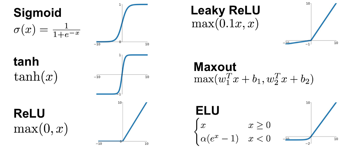
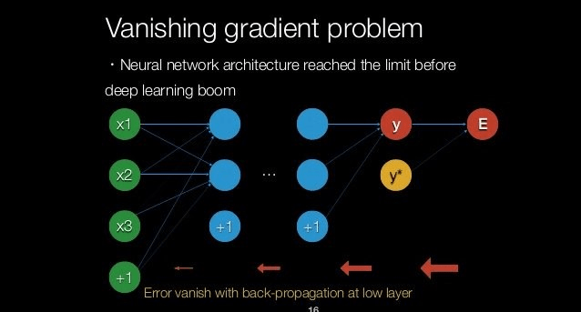
Vanishing Gradient
when the gradients are very small, they can diminish as they are propagated back through the network, leading to minimal or no updates to the weights in the initial layers.
Activation functions like the sigmoid or hyperbolic tangent (tanh) have gradients that are in the range of 0 to 0.25 for sigmoid and -1 to 1 for tanh: the gradients of the loss function with respect to the parameters can become very small
Slow and stalled learning
see link
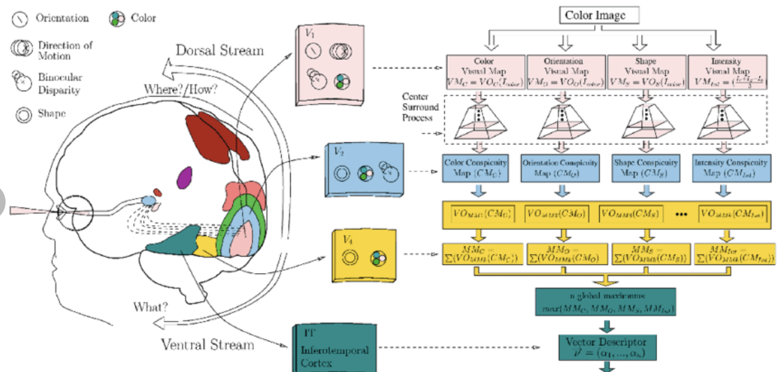
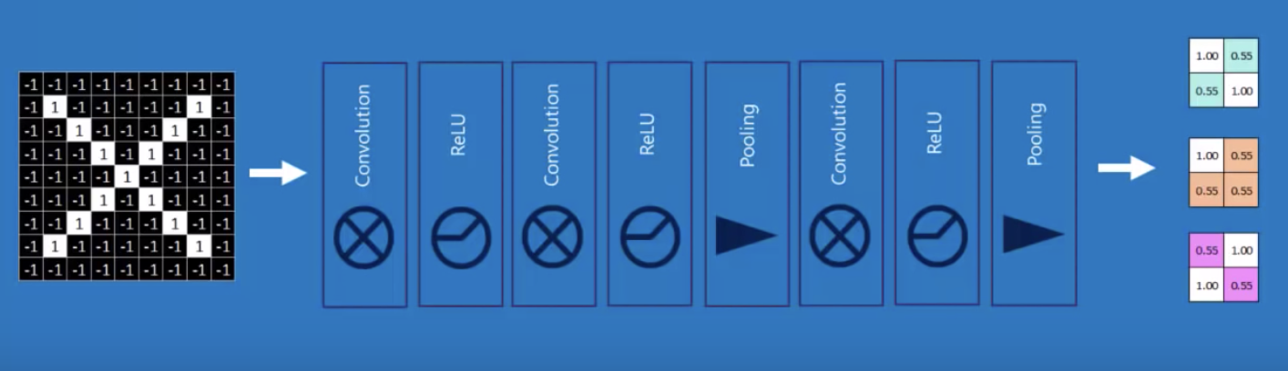
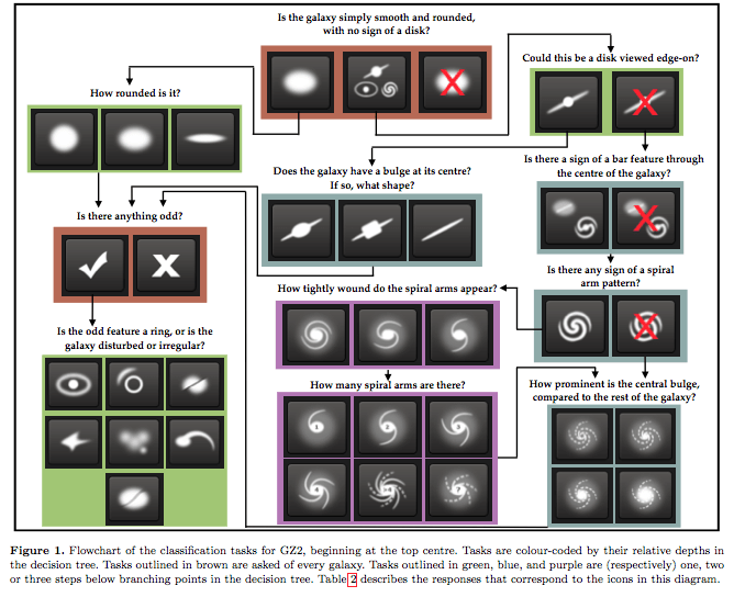
Convolutional Neural Nets
@akumadog
The visual cortex learns hierarchically: first detects simple features, then more complex features and ensembles of features
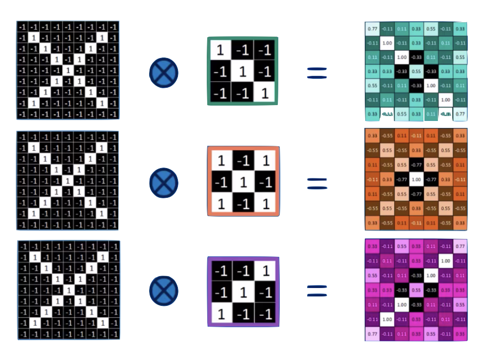
Convolution
Convolution
convolution is a mathematical operator on two functions
f and g
that produces a third function
f x g
expressing how the shape of one is modified by the other.
o
Convolution Theorem
fourier transform
two images.
model.add(Conv2D(64, kernel_size=(3, 3), activation='relu'))
| -1 | -1 | -1 | -1 | -1 |
|---|---|---|---|---|
| -1 | -1 | -1 | ||
| -1 | -1 | -1 | -1 | |
| -1 | -1 | -1 | ||
| -1 | -1 | -1 | -1 | -1 |
1
1
1
1
1
1
1
1
1
| -1 | -1 | -1 | -1 | -1 |
|---|---|---|---|---|
| -1 | -1 | -1 | -1 | -1 |
| -1 | -1 | -1 | -1 | -1 |
| -1 | -1 | -1 | -1 | -1 |
| -1 | -1 | -1 | -1 | -1 |
model.add(Conv2D(64, kernel_size=(3, 3), activation='relu'))
| 1 | -1 | -1 |
| -1 | 1 | -1 |
| -1 | -1 | 1 |
1
1
1
1
1
| -1 | -1 | -1 | -1 | -1 |
|---|---|---|---|---|
| -1 | -1 | -1 | ||
| -1 | -1 | -1 | -1 | |
| -1 | -1 | -1 | ||
| -1 | -1 | -1 | -1 | -1 |
| -1 | -1 | 1 |
| -1 | 1 | -1 |
| 1 | -1 | -1 |
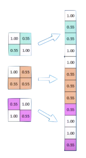
feature maps
model.add(Conv2D(64, kernel_size=(3, 3), activation='relu'))
1
1
1
1
1
convolution
| -1 | -1 | -1 | -1 | -1 |
|---|---|---|---|---|
| -1 | -1 | -1 | ||
| -1 | -1 | -1 | -1 | |
| -1 | -1 | -1 | ||
| -1 | -1 | -1 | -1 | -1 |
| 1 | -1 | -1 |
| -1 | 1 | -1 |
| -1 | -1 | 1 |
model.add(Conv2D(64, kernel_size=(3, 3), activation='relu'))
1
1
1
1
1
| -1 | -1 | -1 | -1 | -1 |
|---|---|---|---|---|
| -1 | -1 | -1 | ||
| -1 | -1 | -1 | -1 | |
| -1 | -1 | -1 | ||
| -1 | -1 | -1 | -1 | -1 |
| 1 | -1 | -1 |
| -1 | 1 | -1 |
| -1 | -1 | 1 |
| 1 | -1 | -1 |
| -1 | 1 | -1 |
| -1 | -1 | 1 |
| 7 | ||
|---|---|---|
=
model.add(Conv2D(64, kernel_size=(3, 3), activation='relu'))
1
1
1
1
1
| -1 | -1 | -1 | -1 | -1 |
|---|---|---|---|---|
| -1 | -1 | -1 | ||
| -1 | -1 | -1 | -1 | |
| -1 | -1 | -1 | ||
| -1 | -1 | -1 | -1 | -1 |
| 1 | -1 | -1 |
| -1 | 1 | -1 |
| -1 | -1 | 1 |
| 1 | -1 | -1 |
| -1 | 1 | -1 |
| -1 | -1 | 1 |
| 7 | -3 | |
|---|---|---|
=
model.add(Conv2D(64, kernel_size=(3, 3), activation='relu'))
1
1
1
1
1
| -1 | -1 | -1 | -1 | -1 |
|---|---|---|---|---|
| -1 | -1 | -1 | ||
| -1 | -1 | -1 | -1 | |
| -1 | -1 | -1 | ||
| -1 | -1 | -1 | -1 | -1 |
| 1 | -1 | -1 |
| -1 | 1 | -1 |
| -1 | -1 | 1 |
| 1 | -1 | -1 |
| -1 | 1 | -1 |
| -1 | -1 | 1 |
| 7 | -3 | 3 |
|---|---|---|
=
model.add(Conv2D(64, kernel_size=(3, 3), activation='relu'))
1
1
1
1
1
| -1 | -1 | -1 | -1 | -1 |
|---|---|---|---|---|
| -1 | -1 | -1 | ||
| -1 | -1 | -1 | -1 | |
| -1 | -1 | -1 | ||
| -1 | -1 | -1 | -1 | -1 |
| 1 | -1 | -1 |
| -1 | 1 | -1 |
| -1 | -1 | 1 |
| 1 | -1 | -1 |
| -1 | 1 | -1 |
| -1 | -1 | 1 |
| 7 | -1 | 3 |
|---|---|---|
| ? | ||
=
model.add(Conv2D(64, kernel_size=(3, 3), activation='relu'))
1
1
1
1
1
| -1 | -1 | -1 | -1 | -1 |
|---|---|---|---|---|
| -1 | -1 | -1 | ||
| -1 | -1 | -1 | -1 | |
| -1 | -1 | -1 | ||
| -1 | -1 | -1 | -1 | -1 |
| 1 | -1 | -1 |
| -1 | 1 | -1 |
| -1 | -1 | 1 |
| 1 | -1 | -1 |
| -1 | 1 | -1 |
| -1 | -1 | 1 |
| 7 | -1 | 3 |
|---|---|---|
| ? | ? | |
=
model.add(Conv2D(64, kernel_size=(3, 3), activation='relu'))
1
1
1
1
1
| -1 | -1 | -1 | -1 | -1 |
|---|---|---|---|---|
| -1 | -1 | -1 | ||
| -1 | -1 | -1 | -1 | |
| -1 | -1 | -1 | ||
| -1 | -1 | -1 | -1 | -1 |
| 1 | -1 | -1 |
| -1 | 1 | -1 |
| -1 | -1 | 1 |
| 7 | -1 | 3 |
|---|---|---|
| -3 | ||
=
input layer
feature map
convolution layer
model.add(Conv2D(64, kernel_size=(3, 3), activation='relu'))
1
1
1
1
1
| -1 | -1 | -1 | -1 | -1 |
|---|---|---|---|---|
| -1 | -1 | -1 | ||
| -1 | -1 | -1 | -1 | |
| -1 | -1 | -1 | ||
| -1 | -1 | -1 | -1 | -1 |
| 1 | -1 | -1 |
| -1 | 1 | -1 |
| -1 | -1 | 1 |
| 7 | -3 | 3 |
| -3 | 5 | -3 |
| 3 | -1 | 7 |
=
input layer
feature map
convolution layer
the feature map is "richer": we went from binary to R
and it is reminiscent of the original layer
7
5
7
model.add(Conv2D(64, kernel_size=(3, 3), activation='relu'))
Convolve with different feature: each neuron is 1 feature
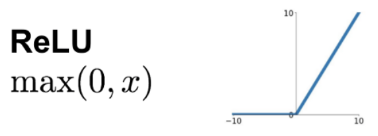
ReLu
| 7 | -3 | 3 |
| -3 | 5 | -3 |
| 3 | -1 | 7 |
7
5
7
ReLu: normalization that replaces negative values with 0's
| 7 | 0 | 3 |
| 0 | 5 | 0 |
| 3 | 0 | 7 |
7
5
7
model.add(Conv2D(64, kernel_size=(3, 3), activation='relu'))
Max-Pool
MaxPooling: reduce image size, generalizes result
| 7 | 0 | 3 |
| 0 | 5 | 0 |
| 0 | 0 | 7 |
7
5
7
MaxPooling: reduce image size, generalizes result
| 7 | 0 | 3 |
| 0 | 5 | 0 |
| 3 | 0 | 7 |
7
5
7
2x2 Max Poll
| 7 | 5 |
MaxPooling: reduce image size, generalizes result
| 7 | 0 | 3 |
| 0 | 5 | 0 |
| 3 | 0 | 7 |
7
5
7
2x2 Max Poll
| 7 | 5 |
| 5 |
MaxPooling: reduce image size, generalizes result
| 7 | 0 | 3 |
| 0 | 5 | 0 |
| 3 | 0 | 7 |
7
5
7
2x2 Max Poll
| 7 | 5 |
| 5 | 7 |
MaxPooling: reduce image size & generalizes result
By reducing the size and picking the maximum of a sub-region we make the network less sensitive to specific details
model.add(MaxPooling2D(pool_size=(2, 2)))from keras.models import Sequential
from keras.layers import Dense, Dropout, Flatten
from keras.layers import Conv2D, MaxPooling2D
model = Sequencial()
model.add(Conv2D(32, kernel_size=(10, 10),
activation='relu',
input_shape=input_shape))
model.add(Conv2D(64, kernel_size=(3, 3), activation='relu'))
model.add(MaxPooling2D(pool_size=(2, 2)))
model.add(Conv2D(32, kernel_size=(3, 3), activation='relu'))
model.add(MaxPooling2D(pool_size=(2, 2)))x
O
last hidden layer
output layer
from keras.models import Sequential
from keras.layers import Dense, Dropout, Flatten
from keras.layers import Conv2D, MaxPooling2D
model = Sequencial()
model.add(Conv2D(32, kernel_size=(10, 10),
                 activation='relu',
                 input_shape=input_shape))
model.add(Conv2D(64, kernel_size=(3, 3), activation='relu'))
model.add(MaxPooling2D(pool_size=(2, 2)))
model.add(Conv2D(32, kernel_size=(3, 3), activation='relu'))
model.add(MaxPooling2D(pool_size=(2, 2)))
model.add(Flatten())
model.add(Dense(128, activation='relu'))
model.add(Dense(2, activation='softmax'))Stack multiple convolution layers
Minibatch
&
Dropout
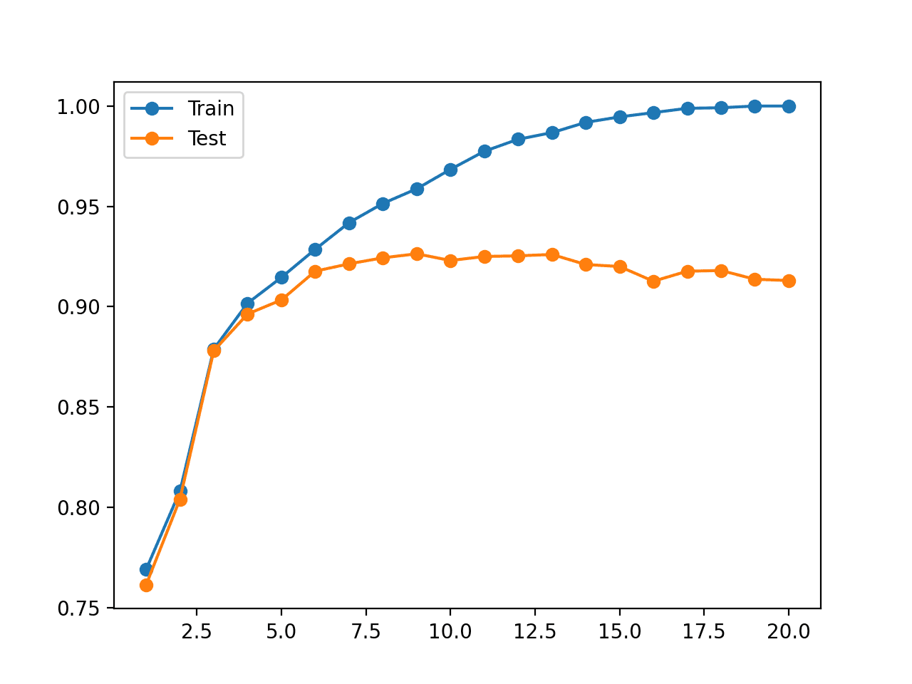
What are the symptoms
How can we fix it?
model performance (accuracy)
model performance (accuracy)
tree depth
tree depth
ANN training epochs
Split your training set into many smaller subsets and train on each small set separately
Dropout
Artificially remove some neurons for different minibatches to avoid overfitting
output
from keras.models import Sequential
from keras.layers import Dropout
model.add(Dropout(0.5))what is the simplest classifier you can build for this dataset ?
what is the accuracy?
x
y
If your dataset is imbalanced (more of one class than the other)
your model will learn that it is better to guess the most common class
this will contaminate the prediction
what is the simplest classifier you can build for this dataset ?
what is the accuracy?
x
y
If your dataset is imbalanced (more of one class than the other)
Architecture components: neurons, activation function
Single layer NN: perceptrons
Deep NN:
Convolutional NN
Training an NN:
By federica bianco
convolutional neural networks


