


federica bianco PRO
astro | data science | data for good
dr.federica bianco | fbb.space | fedhere | fedhere
k-NN
this slide deck
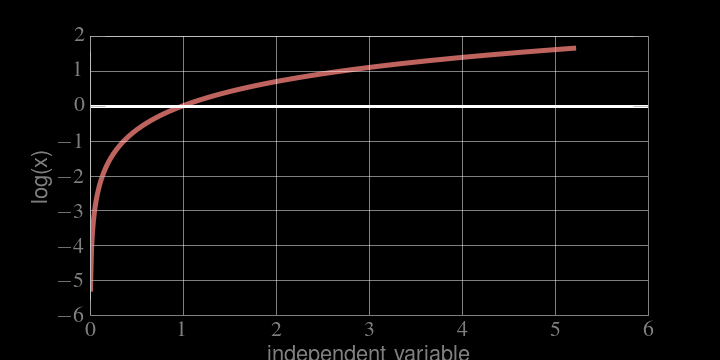
MONOTONICALLY INCREASING
if x grows, log(x) grows, if x decreases, log(x) decreases
the location of the maximum is the same!
SUPPORT :
MONOTONICALLY INCREASING
SUPPORT :
Not a problem cause L like P is positive defined
MONOTONICALLY INCREASING
not part of the model
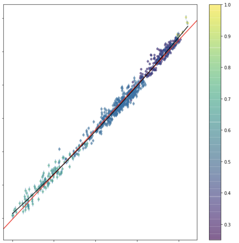
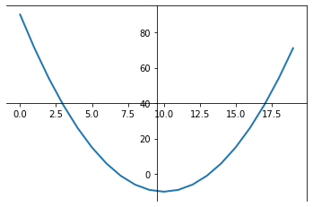
think about the likelihood surfece...
you want to explore the surface and find a peak
param
likelihood
100
200
-100
-200
-log(likelihood)
param
think about the likelihood surfece...
you want to explore the surface and find a peak
slope
intercept
think about the likelihood surfece...
you want to explore the surface and find a peak
possible issues:
- how do I efficiently explore the whole surface?
- how do I explore the WHOLE survey at all?
- how do I avoid getting stuck in a local minimum (maximum)?
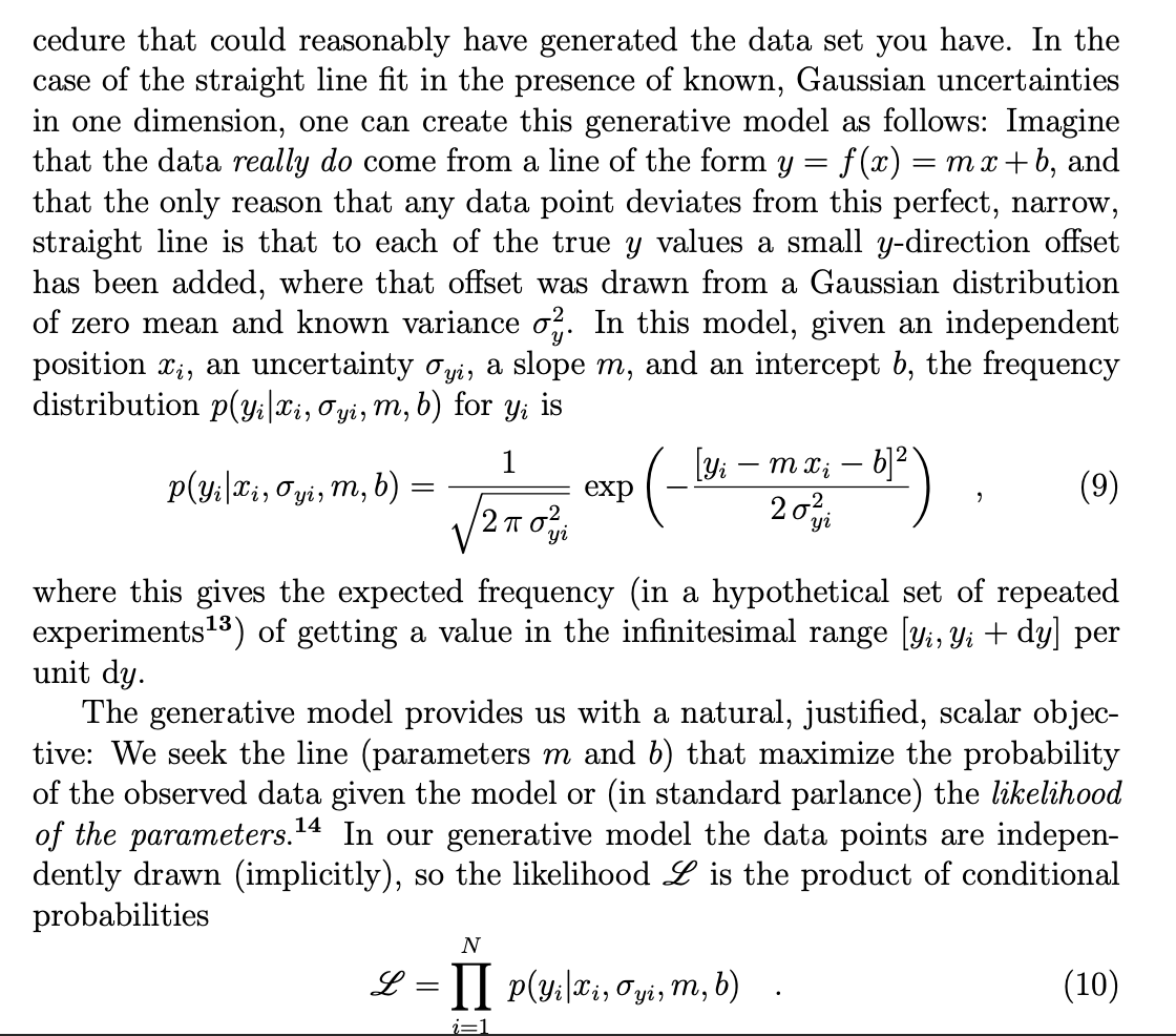
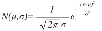
The problem of fitting models to data reduces to finding the
maximum likelihood
of the data given the model
This is effectively done by finding the minimum of the
-log(likelihood)
principles
2.1
the answer truly depends on what you are modeling for and what domain knowledge is available
except:
William of Ockham (logician and Franciscan friar) 1300ca
but probably to be attributed to John Duns Scotus (1265–1308)
“Complexity needs not to be postulated without a need for it”
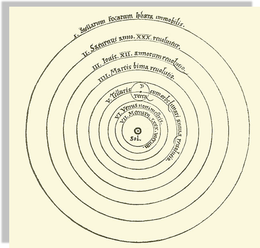
Peter Apian, Cosmographia, Antwerp, 1524 from Edward Grant,
"Celestial Orbs in the Latin Middle Ages", Isis, Vol. 78, No. 2. (Jun., 1987).
Geocentric models are intuitive:
from our perspective we see the Sun moving, while we stay still
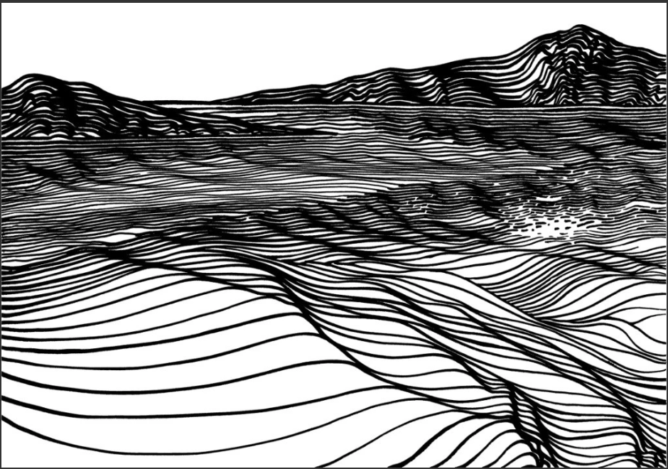
the earth is round,
and it orbits around the sun
As observations improve
this model can no longer fit the data!
not easily anyways...
the earth is round,
and it orbits around the sun
Encyclopaedia Brittanica 1st Edition
Dr Long's copy of Cassini, 1777
A new model that is much simpler fit the data just as well
(perhaps though only until better data comes...)
the earth is round,
and it orbits around the sun
Heliocentric model from Nicolaus Copernicus' De revolutionibus orbium coelestium.
William of Ockham (logician and Franciscan friar) 1300ca
but probably to be attributed to John Duns Scotus (1265–1308)
“Complexity needs not to be postulated without a need for it”
William of Ockham (logician and Franciscan friar) 1300ca
but probably to be attributed to John Duns Scotus (1265–1308)
“Complexity needs not to be postulated without a need for it”
“Between 2 theories that perform similarly choose the simpler one”
William of Ockham (logician and Franciscan friar) 1300ca
but probably to be attributed to John Duns Scotus (1265–1308)
“Complexity needs not to be postulated without a need for it”
“Between 2 theories that perform similarly choose the one with fewer parameters”
Since all models are wrong the scientist cannot obtain a "correct" one by excessive elaboration. On the contrary following William of Occam he should seek an economical description of natural phenomena
Since all models are wrong the scientist must be alert to what is importantly wrong.
Science and Statistics George E. P. Box (1976)
Journal of the American Statistical Association, Vol. 71, No. 356, pp. 791-799.
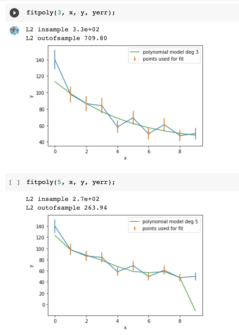
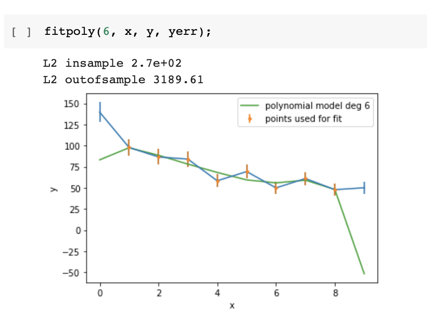
Careful!
Increasing the model's degrees freedom allows a "better fit" in the in-sample set
methods
2.2
HOW DO I CHOOSE A MODEL?
Given two models which is preferable?
Likelihood-ratio tests
likelihood ratio statistics LR
NESTED MODELS : one model contains the other one, e.g.
y= mx + l
is contained in
y=ax**2+ mx + l
statsmodels.model.compare_lr_ratio()
A rigorous answer (in terms of NHST) can be obtained for 2 nested models
This directly answers the question:
“is my more complex model overfitting the data?”
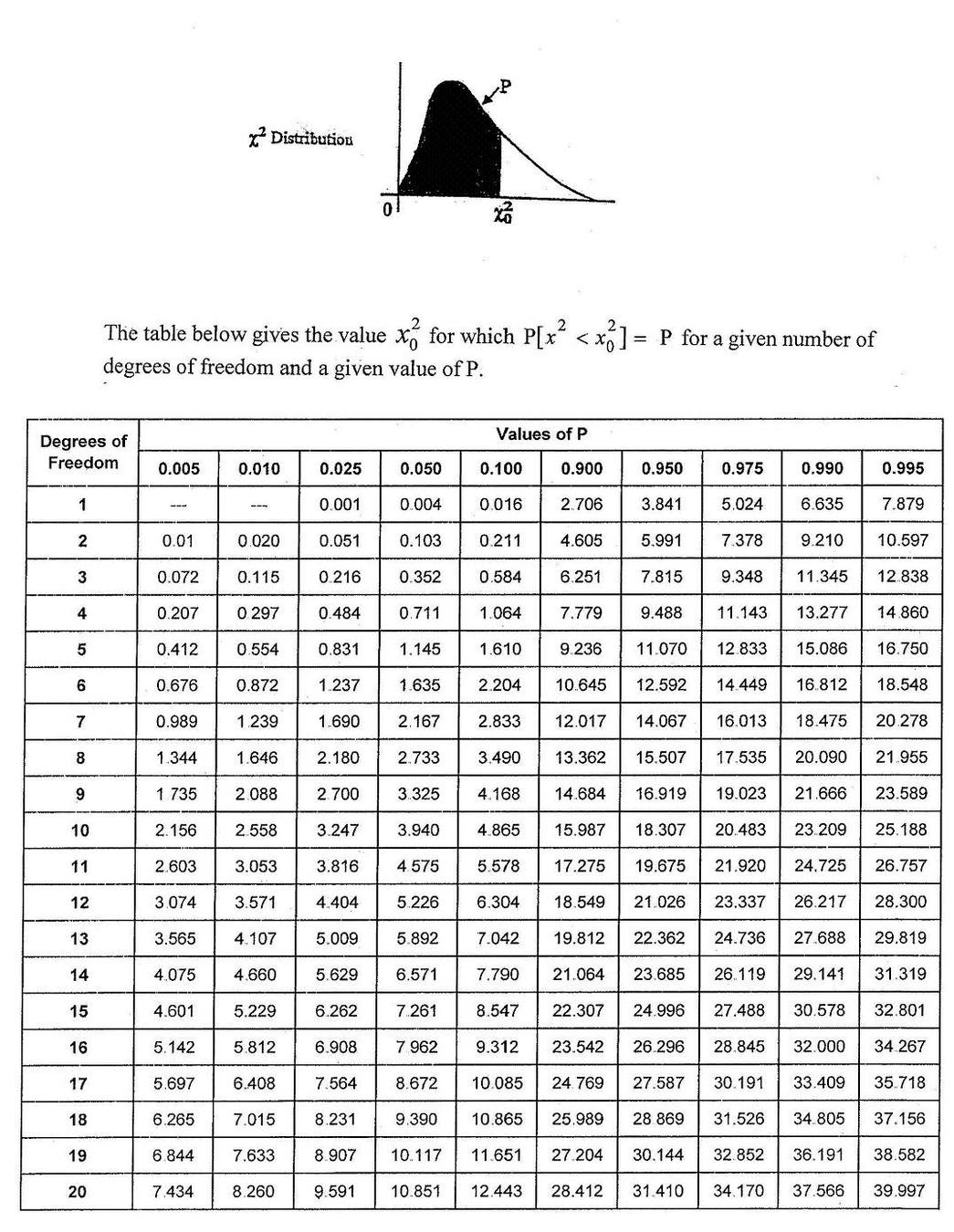
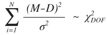
The LR statistics is expected to follow a χ^2 distrbution under the Null Hypothesis that the simpler model is preferable
HOW DO I CHOOSE A MODEL?
Given two models which is preferable?
Likelihood-ratio tests
NESTED MODELS : one model contains the other one, e.g.
y= mx + l
is contained in
y=ax**2+ mx + l
A rigorous answer (in terms of NHST) can be obtained for 2 nested models
This directly answers the question:
“is my more complex model overfitting the data?”
The LR statistics is expected to follow a χ^2 distrbution under the Null Hypothesis that the simpler model is preferable
from scipy.stats.distributions import chi2
def likelihood_ratio(llmin, llmax):
    return(-2*(llmax-llmin))

LR = likelihood_ratio(L1,L2)

p = chi2.sf(LR, dof)
# dof: difference in number of parameters
print ('p: %.30f' % p)
# LR is chi squared distributed:
# p represents the probability that this result
# (or a more extreme result than this)
# would happen by chance
HOW DO I CHOOSE A MODEL?
Given two models which is preferable?
Likelihood-ratio tests
likelihood ratio statistics LR
statsmodels.model.compare_lr_ratio()
The LR statistics is expected to follow a χ^2 distrbution under the Null Hypothesis that the simpler model is preferable
difference in number of parameters between the 2 models
Shannon 1948: A Mathematical Theory of Communication
a theory to find fundamental limits on signal processing and communication operations such as data compression
model selection is also based on the minimization of a quantity. Several quantities are suitable:
MLD
BIC
Bayese theorem
AIC
Optimism and likelihood maximization on the training set
number of parameters:
Model Complexity
Likelihood: Model Performance.
Akaike information criterion (AIC) .
Based on
where is a family of function (=densities) containing the correct (=true) function and is the set of parameters that maximized the likelihood L
L is the likelihood of the data, k is the number of parameters,
N the number of variables.
number of parameters:
Model Complexity
Likelihood: Model Performance.
"-" sign in front of the log-likelihood: AIC shrinks for better models,
AIC ~ k => is linearly proportional to the number of parameters
Akaike information criterion (AIC) .
Based on
where is a family of function (=densities) containing the correct (=true) function and is the set of parameters that maximized the likelihood L
L is the likelihood of the data, k is the number of parameters,
N the number of observations.
Likelihood: Model Performance.
number of parameters:
Model Complexity
Bayesian information criterion (BIC) .
L is the likelihood of the data, k is the number of parameters,
N the number of observations.
stronger penalization of complexity (as long as N> )
The derivation is very different:
Bayes Factor
Minimum Description Length (MDL) .
negative log-likelihood of the model parameters (θ) and the negative log-likelihood of the target values (y) given the input values (X) and the model parameters (θ).
also: log(L(θ)): number of bits required to represent the model,
log(L(y| X,θ)): number of bits required to represent the predictions on observations
minimize the encoding of the model and its predictions
derived from Shannon's theorem of information
Mathematically similar, though derived from different approaches. All used the same way: the preferred model is the model that minimized the estimator
HOW DO I CHOOSE A MODEL?
Given two models which is preferable?
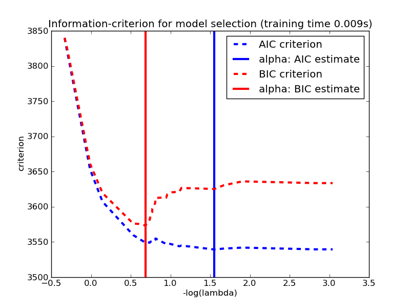
AIC - BIC
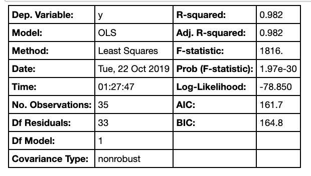
also consider at Akaike and Bayesian Information Criteria for not nested models:
both are returned in a statsmodel fit
A rigorous answer (in terms of NHST) can be obtained for 2 nested models
This directly answers the question:
“is my more complex model overfitting the data?”
The LR statistics is expected to follow a χ^2 distrbution under the Null Hypothesis that the simpler model is preferable
they are calculated combining the likelihood with a penalization for the extra parameters
generally both decrease with increasing increasing likelihood but you would look for the place where they start decreasing slowly as the "sweet spot" for your model
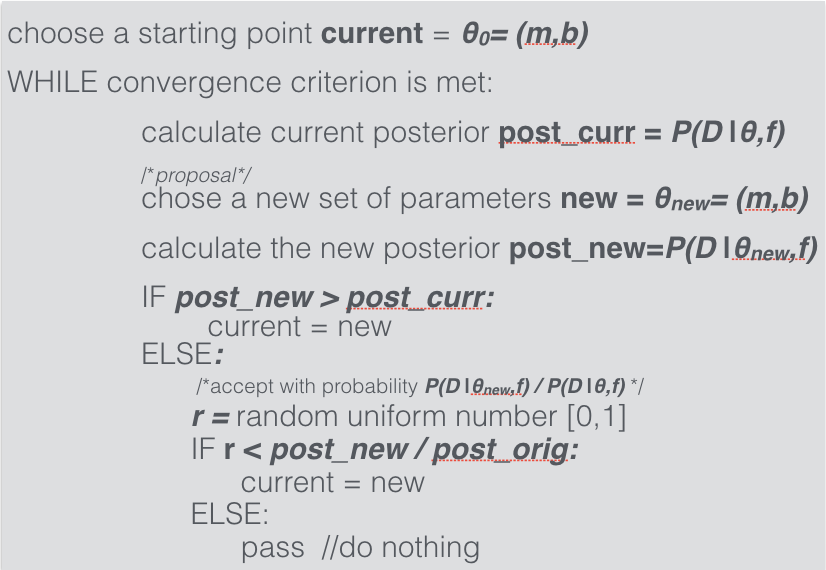
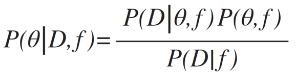
posterior
Goal: sample the posterior distribution
Examples of how to choose the next point
Metropolis-Hasting
Gaussian random walk proposal distribution
choose a random starting point current = θo = (m,b)
WHILE convergence criterion is met:
calculate the current posterior post_curr = P(D| θo,f)
/*proposal*/
draw a new set of parameters new = θnew = (m,b)
calculate the current posterior post_new = P(D| θnew,f)
IF post_new > post_curr:
current = new
ELSE
/*accept with probability P(D| θnew,f)/P(D| θo,f) */
r = random uniform number [0,1]
IF r < post_new / post_curr:
current = new
ELSE
pass //do nothing
posterior
Goal: sample the posterior distribution
Examples of how to choose the next point
Metropolis-Hastings proposal distribution with change along a single direction at a time => always accept
must know the conditional distribution of each variable
posterior
Goal: sample the posterior distribution
Examples of how to choose the next point
Other options:
simulated annealing (good for multimodal)
parallel tempering (good for multimodal)
differential evoution (good for covariant spaces)
posterior
Goal: sample the posterior distribution
Examples of how to choose the next point
affine invariant : EMCEE package
Examples of how to choose the next point
Other options:
simulated annealing (good for multimodal)
parallel tempering (good for multimodal)
differential evoution (good for covariant spaces)
Examples of how to choose the next point
Other options:
Hamiltonian MC: proposing moves to distant states which maintain a high probability of acceptance due to the approximate energy conserving properties of the simulated Hamiltonian
simulated annealing (good for multimodal)
parallel tempering (good for multimodal)
differential evoution (good for covariant spaces)
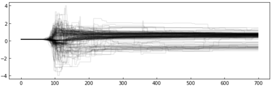
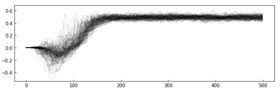
MCMC convergence
MCMC convergence
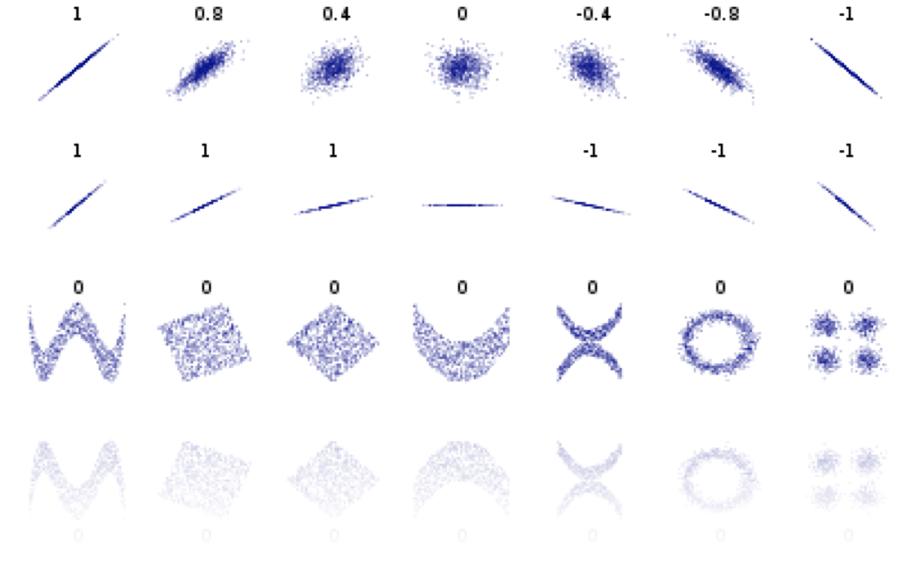
Pearson's test: tests linear correlation
import scipy as sp
print("Pearson's correlation {:.2}, approximate p-value {:.2}".format(
    *sp.stats.pearsonr(x, y)))
Pearson's correlation 0.94, approximate p-value 2.9e-49
Pearson's test
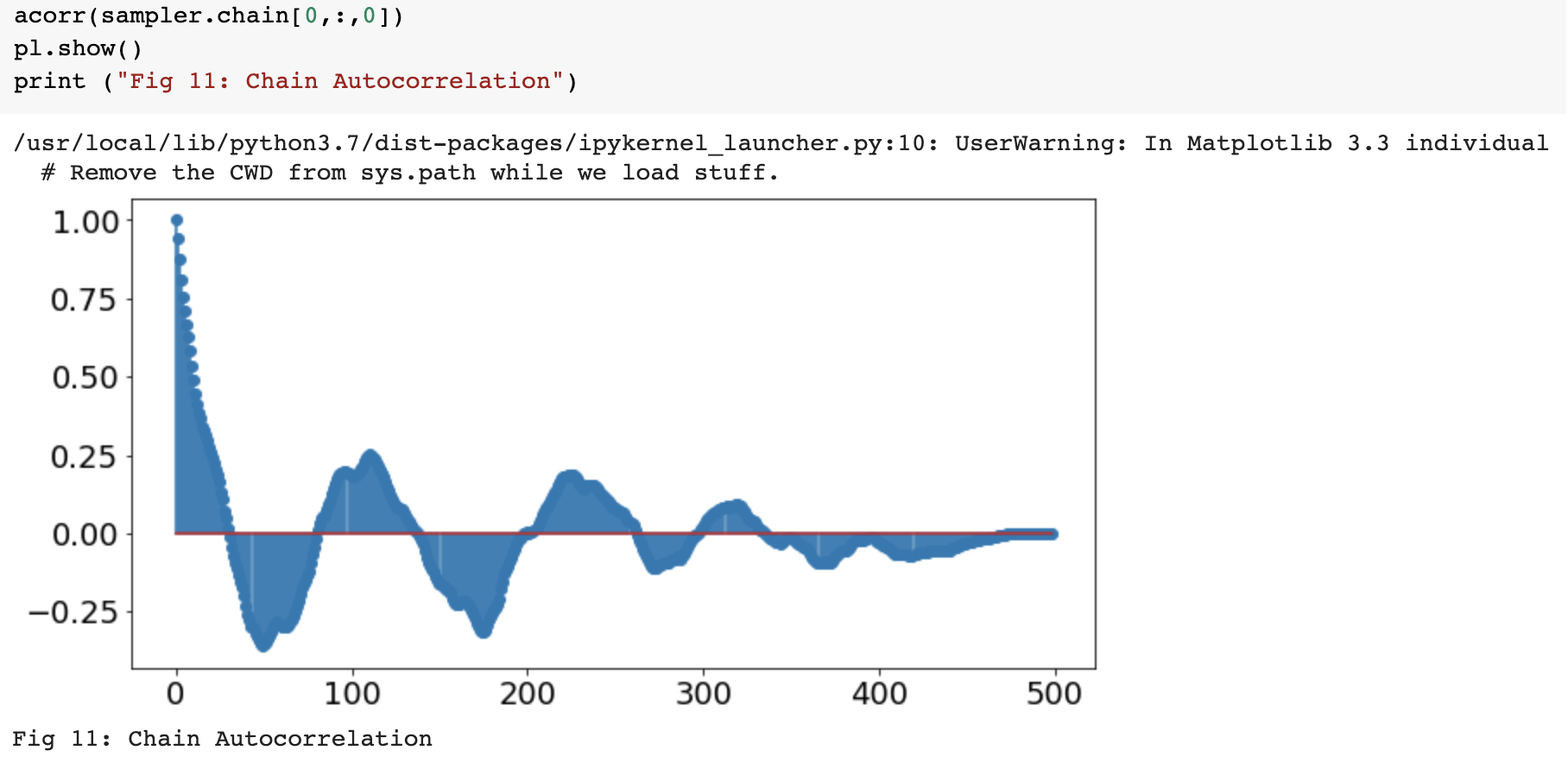
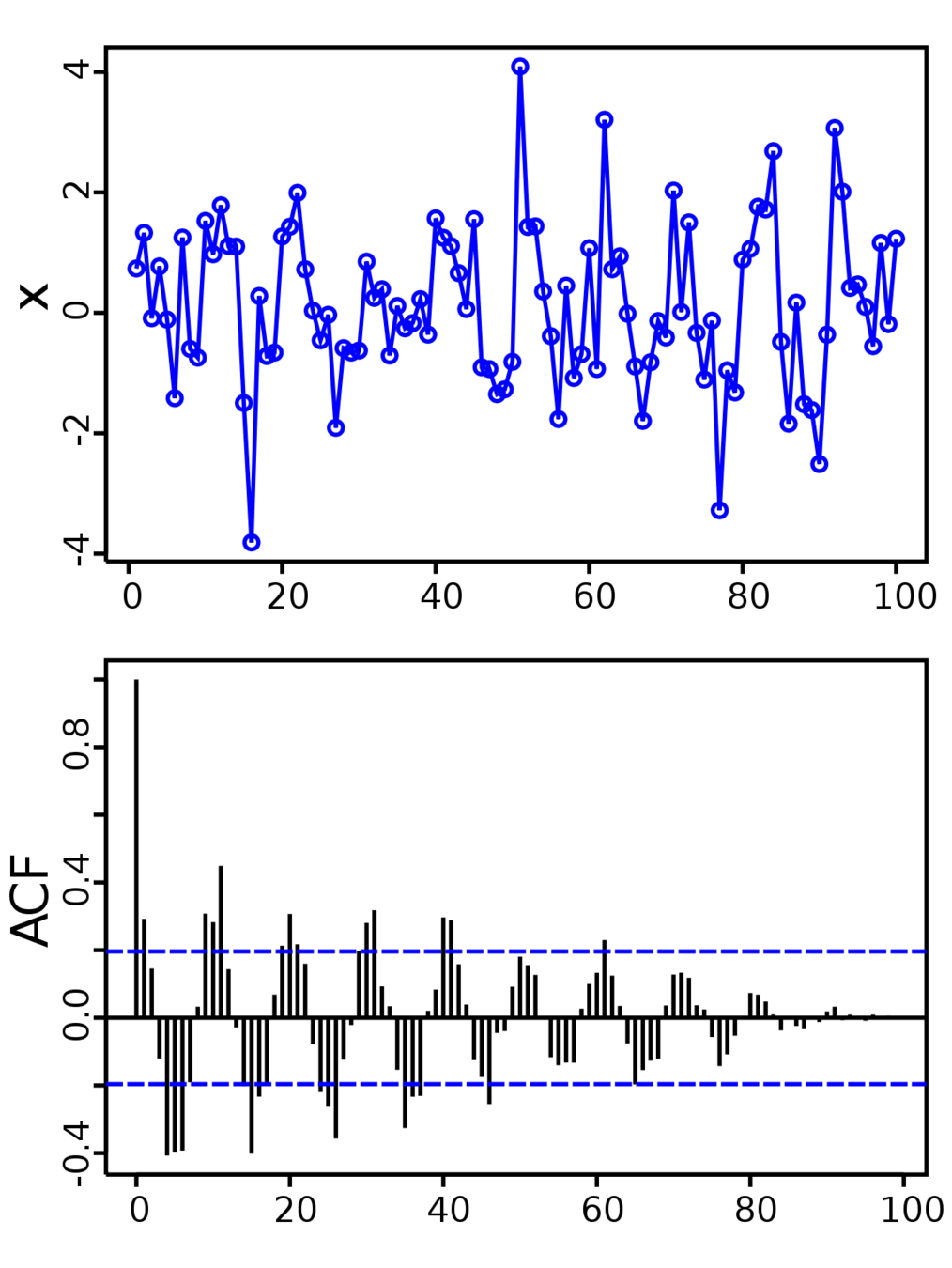
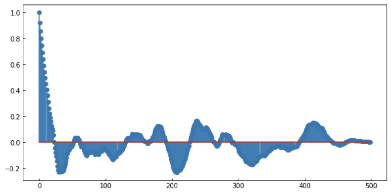
autocorrelation
MCMC convergence
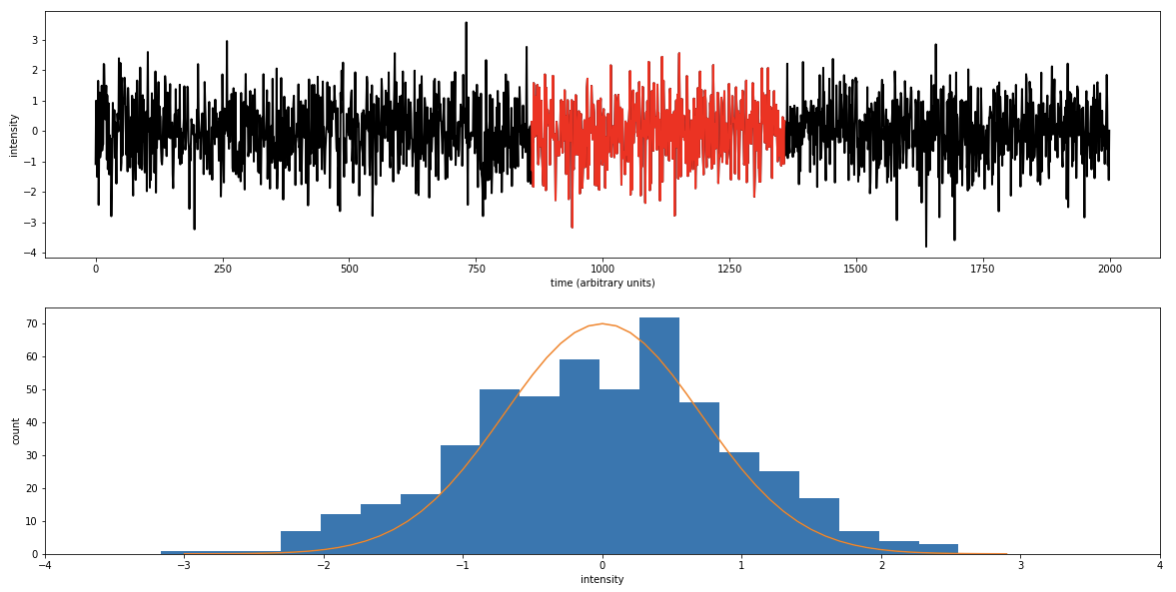
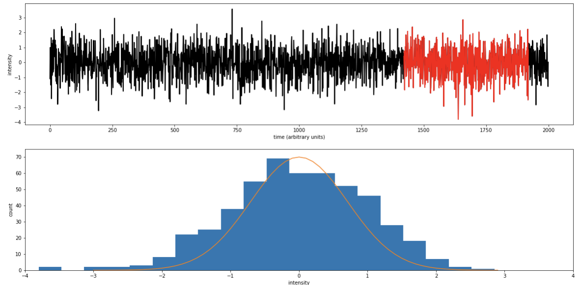
A random variable indexed by time.
For any subset of points in time the dependent variable follows the a probability distribution
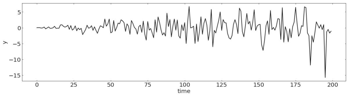
e.g.
pl.figure(figsize=(20,5))
N = 200
np.random.seed(100)
y = np.random.randn(N)
t = np.linspace(0, N, N, endpoint=False)
pl.plot(t, y, lw=2)
pl.xlabel("time")
pl.ylabel("y");
Discrete stochastic process
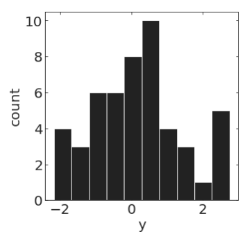
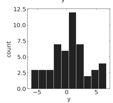
pl.hist(y[20:70])pl.hist(y[100:150])A time series is strictly stationary if for any i and Δt
MCMC convergence
MCMC convergence
MCMC convergence
Stochastic Processes in Science Inference: with the advent of computers (1940s), simulations became a valuable alternative to analytical derivation to solve complex scientific problems, and the only way to solve non-tractable problems. Events that occur with a known probability can be simulated, the possible outcomes would be simulated with a frequency corresponding to the probability.
Applications: Instances of the evolution of a complex systems can be simulated, and from this synthetic (simulated) sample solutions can be generalized as they would from a sample observed from a population:
Physics example: simulate multibody interactions (e.g. asteroids or particles in large systems) or nuclear reaction chains
Urban e.g.. simulate traffic flow to determine the average trip duration instead of measuring many trips to estimate the trip duration,
or a better scheme would be: simulate traffic flow and validate your simulation by comparing the average trip duration for a synthetic sample and from a sample observed from the real system, then simulate proposed changes to traffic to validate and evaluate planning options before implementing them.
Simulations require drawing samples from distributions.
We did not cocer this but it is important - you wont need to do it cause python numpy/scipy does it for you... but you should know this
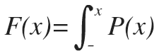
Drawing samples from a distribution can be done directly if the probability PDF P(X) can be integrated analytically to find a CDF F(x) and if this CDF is invertible (F-1(u) can be calculated analytically) . The algorithm is:
If F(x) or F-1(u) cannot be calculated analytically Rejection Sampling allows to sample from the desired P(x) . The algorithm is:
If your proposal distribution is poorly chosen (much higher than P(x) in some regions) this can be an extremely wasteful process. The higher the problem dimensionality the more this issue becomes a concern. Alternatives include Importance sampling where the integral of the PDF is performed numerically with a correction for every x given by the ratio of P(x) to Q(x)
Markovian processes: A process is Markovian if the next state of the system is determined stochastically as a perturbation of the current state of the system, and only the current state of the system, i.e. the system has no memory of earlier states (a memory-less process).
A state being a stochastic perturbation of the previous state means that given the conditions of the state at time t (e.g. A(t) = (position+velocity) ) the next set of conditions A(t+1) (updated position+velocity) will be drawn from a distribution related to the earlier state. For example the next velocity can be a sample from a Gaussian distribution with mean equal to the current velocity. A(t+1) ~ N(A(t), s)
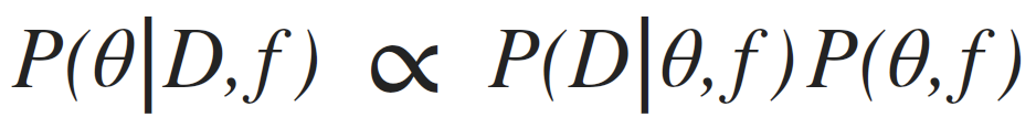
Bayes theorem: relates observed data to proposed models by allowing to calculate the posterior distribution of model parameters for a given prior and observed dataset (see glossary for term definition).
Posterior(data, model-parameters) = Likelihood(data, model-parameters) * Prior(model-parameters)
Evidence(data)
Markov Chain Monte Carlo: Is a method to sample a parameter space that is based on Bayes theorem. The MCMC samples the joint posterior of the parameters in the model (up to a constant, the evidence, probability of observing your data under any model parameter choice, which is generally not calculable). Thus we can get posterior median, confidence intervals, covariance, etc… The algorithm is:
1. starting at some location in the parameter space propose a new location as a Markovian perturbation of the current location
2. if the proposal posterior is better than the posterior at the current location update your position (and save the new position in the chain)
3. if the proposal posterior is worse than the posterior at the current location update your position with some probability α
The choice of the proposal distribution and rule α for accepting the new step in the chain have to satisfy the ergodic condition, that is: given enough time the entire parameter space would be sampled. (Detailed Balance is a sufficient condition for ergodicity)
If the chain is Markovian and the proposal distribution is ergodic the entire parameter space is sample, given enough time, with sampling frequency proportional to the posterior distribution
Different MCMC algorithms: while all MCMC algorithm share the structure above the choice of proposal and the acceptance probability are different for different MCMC algorithms.
Metropolis Hastings MCMC is the first and most common MCMC with acceptance proportional to the ratio of posteriors: α~posteriorNew/posteriorCurrent. This becomes problematic when the posterior has multiple peaks (may not explore them all) or parameter are highly covariant (may take a very long time to converge)
Convergence: It is crucial to confirm that your chains have converged and your parameter space is properly sampled, but it is also very difficult to do it. Methods include checking for stationarity of the chain means and low auto correlation in the chains. The beginning of the chain is typically removed as the chains require a minimum number of steps to move away from the initial position effectively.
(under proper assumption) follows a χ2 distribution
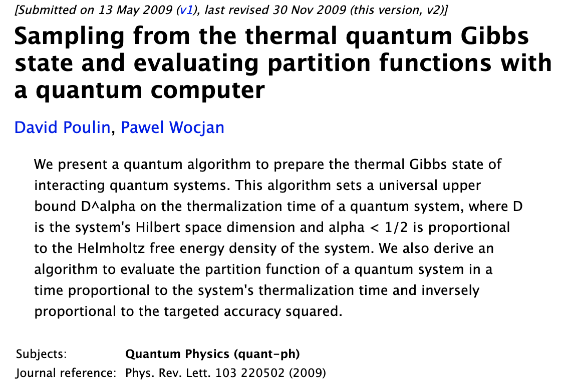
Ensemble samplers with affine invariance
Jonathan Goodman and Jonathan Weare 2010
Bill Press+ 1992 (+)
Information Theory, Inference, and Learning Algorithms
David J.C. MacKay, 2003
Slides on sampling from distributions
Paul E. Johnson 2015
Bill Press (Numerical Recipes) Video
proving how Metropolis-Hastings sutisfied Detail Balance
provides high level discussion, references, suggestion on parameter choices
D. Foreman-Mackey, D. Hogg, D. Lang, J. Goodman+ 2012
3
Machine Learning
unsupervised learning
identify features and create models that allow to understand structure in the data
unsupervised learning
identify features and create models that allow to understand structure in the data
supervised learning
extract features and create models that allow prediction where the correct answer is known for a subset of the data
Calculate the distance d to all known objects

Select the k closest objects

Assign the most common among the k classes:
# k = 1
d = distance(x, trainingset)
C(x) = C(trainingset[argmin(d)])Calculate the distance d to all known objects Select the k closest objects
Classification:
Assign the most common among the k classes
Regression:
Predict the average (median) of the k target values
Good
non parametric
very good with large training sets
Cover and Hart 1967: As n→∞, the 1-NN error is no more than twice the error of the Bayes Optimal classifier.
Good
non parametric
very good with large training sets
Cover and Hart 1967: As n→∞, the 1-NN error is no more than twice the error of the Bayes Optimal classifier.
Let xNN be the nearest neighbor of x.
For n→∞, xNN→x(t) => dist(xNN,x(t))→0
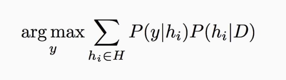
Theorem: e[C(x(t)) = C(xNN)]< e_BayesOpt
e_BayesOpt = argmaxy P(y|x)
Proof: assume P(y|xt) = P(y|xNN)
(always assumed in ML)
eNN = P(y|x(t)) (1−P(y|xNN)) + P(y|xNN) (1−P(y|x(t))) ≤
(1−P(y|xNN)) + (1−P(y|x(t))) =
2 (1−P(y|x(t)) = 2ϵBayesOpt,
Good
non parametric
very good with large training sets
Not so good
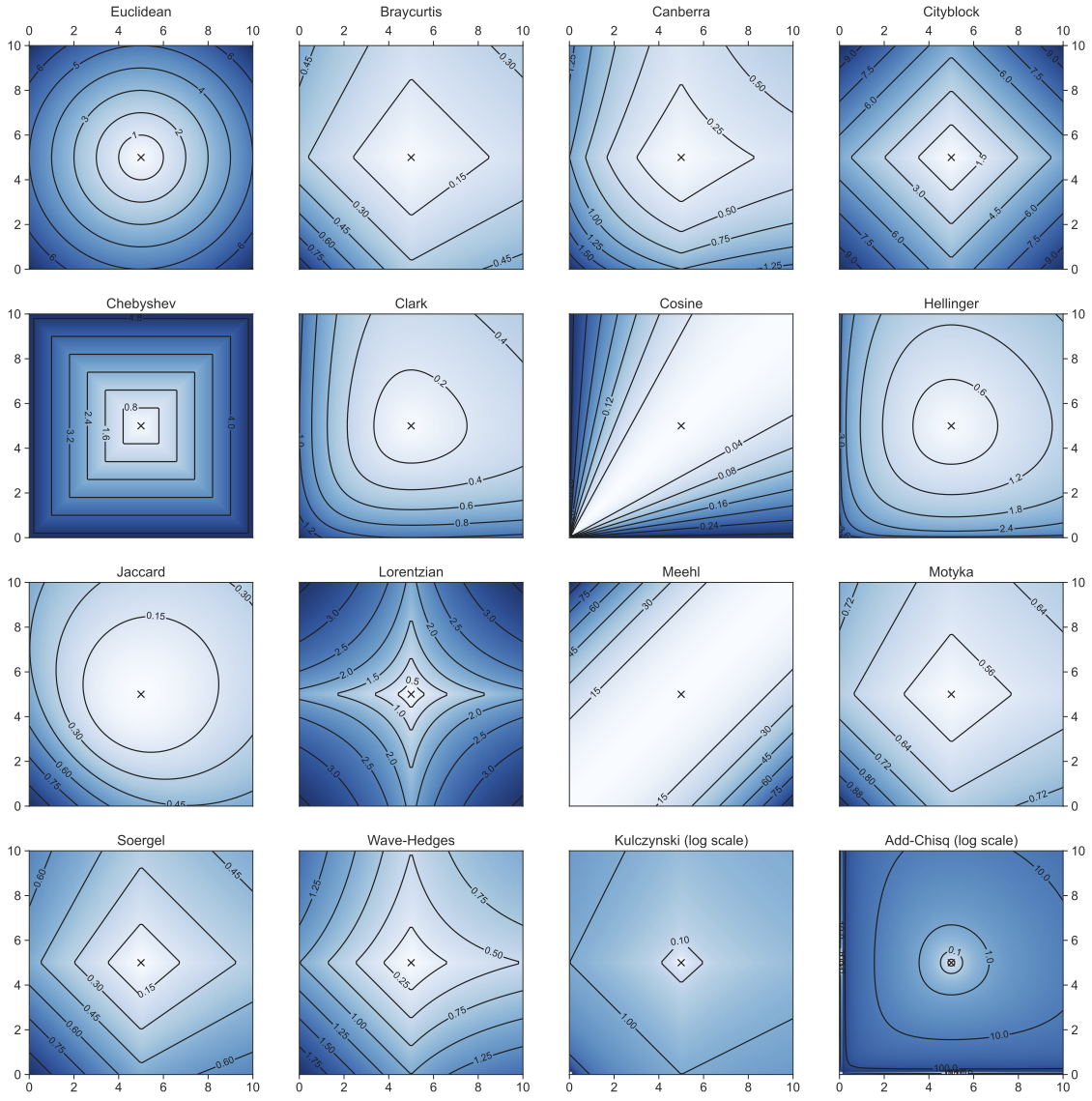
it is only as good as the distance metric
If the similarity in feature space reflect similarity in label then it is perfect!
poor if training sample is sparse
poor with outliers
Wine Example
PROS:
Because the model does not need to provide a global optimization the classification is "on-demand".
This is ideal for recommendation systems: think of Netflix and how it provides recommendations based on programs you have watched in the past.
CONS:
Need to store the entire training dataset (cannot model data to reduce dimensionality).
Training==evaluation => there is no possibility to frontload computational costs
Evaluation on demand, no global optimization - doesn’t learn a discriminative function from the training data but “memorizes” the training dataset instead.
By federica bianco
MCMC


