


federica bianco PRO
astro | data science | data for good
dr.federica bianco | fbb.space | fedhere | fedhere
Clustering
what is machine learning
classification
prediction
feature selection
supervised learning
understanding structure
organizing/compressing data
anomaly detection dimensionality reduction
unsupervised learning
understand structure of feature space
prediction based on examples (inferential AI)
generate new instances (generative AI)
=> second order purpose | feature importance
[Machine Learning is the] field of study that gives computers the ability to learn without being explicitly programmed. Arthur Samuel, 1959
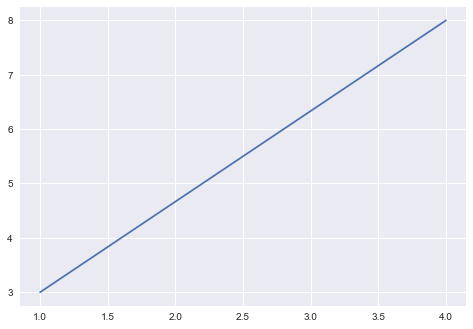
model
parameters:
slope, intercept
data
ML: any model with parameters learnt from the data
[Machine Learning is the] field of study that gives computers the ability to learn without being explicitly programmed. Arthur Samuel, 1959
model
parameters:
slope, intercept
data
ML: any model with parameters learnt from the data
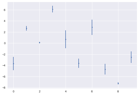
Via minimization of a loss function
Loss function is "distance" between known and predicted values of the target variable
supervised learning
????
unsupervised learning
why
understand structure of feature space
- dimensionality reduction
- anomaly detection
(e.g. image compression)
should be interpretable:
why?
predictive policing,
selection of conference participants.
ethical implications
should be interpretable:
prective policing,
selection of conference participants.
why the model made a choice?
which feature mattered?
why?
ethical implications
causal connection
should be interpretable:
ethical implications
ML model have parameters and hyperparameters
parameters: the model optimizes based on the data
hyperparameters: chosen by the model author, could be based on domain knowledge, other data, guessed (?!).
e.g. the shape of the polynomial
observed features:
(x, y)
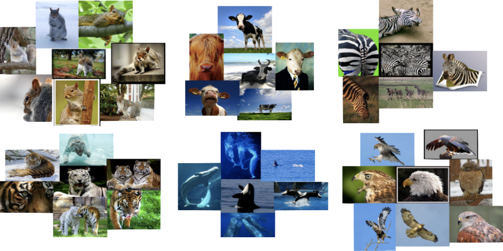
GOAL: partitioning data in maximally homogeneous,
maximally distinguished subsets.
x
y
all features are observed for all objects in the sample
(x, y)
how should I group the observations in this feature space?
e.g.: how many groups should I make?
x
y
internal criterion:
members of the cluster should be similar to each other (intra cluster compactness)
external criterion:
objects outside the cluster should be dissimilar from the objects inside the cluster
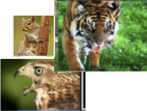
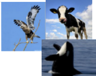
tigers
wales
raptors
zoologist's clusters
orange/green
black/white/blue
internal criterion:
members of the cluster should be similar to each other (intra cluster compactness)
external criterion:
objects outside the cluster should be dissimilar from the objects inside the cluster
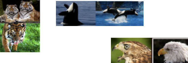
photographer's clusters
how you define similarity/distance
internal criterion:
members of the cluster should be similar to each other (intra cluster compactness)
external criterion:
objects outside the cluster should be dissimilar from the objects inside the cluster
Scalability (naive algorithms are Np hard)
Ability to deal with different types of attributes
Discovery of clusters with arbitrary shapes
Minimal requirement for domain knowledge
Deals with noise and outliers
Insensitive to order
Allows incorporation of constraints
Interpretable
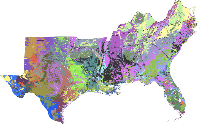
A Spatial Clustering Technique for the Identification of Customizable Ecoregions
William W. Hargrove and Robert J. Luxmoore
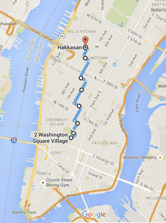
thinking about distances spatially helps intuition
but exercise in abstracting these distances to non-spatial features
A Spatial Clustering Technique for the Identification of Customizable Ecoregions
William W. Hargrove and Robert J. Luxmoore
50-year mean monthly temperature, 50-year mean monthly precipitation, elevation, total plant-available water content of soil, total organic matter in soil, and total Kjeldahl soil nitrogen
Minkowski family of distances
Minkowski family of distances
N features (dimensions)
i,j objects
Minkowski family of distances
N features (dimensions)
properties:
Minkowski family of distances
Manhattan: p=1
features: x, y
Minkowski family of distances
Manhattan: p=1
features: x, y
Minkowski family of distances
Euclidean: p=2
features: x, y
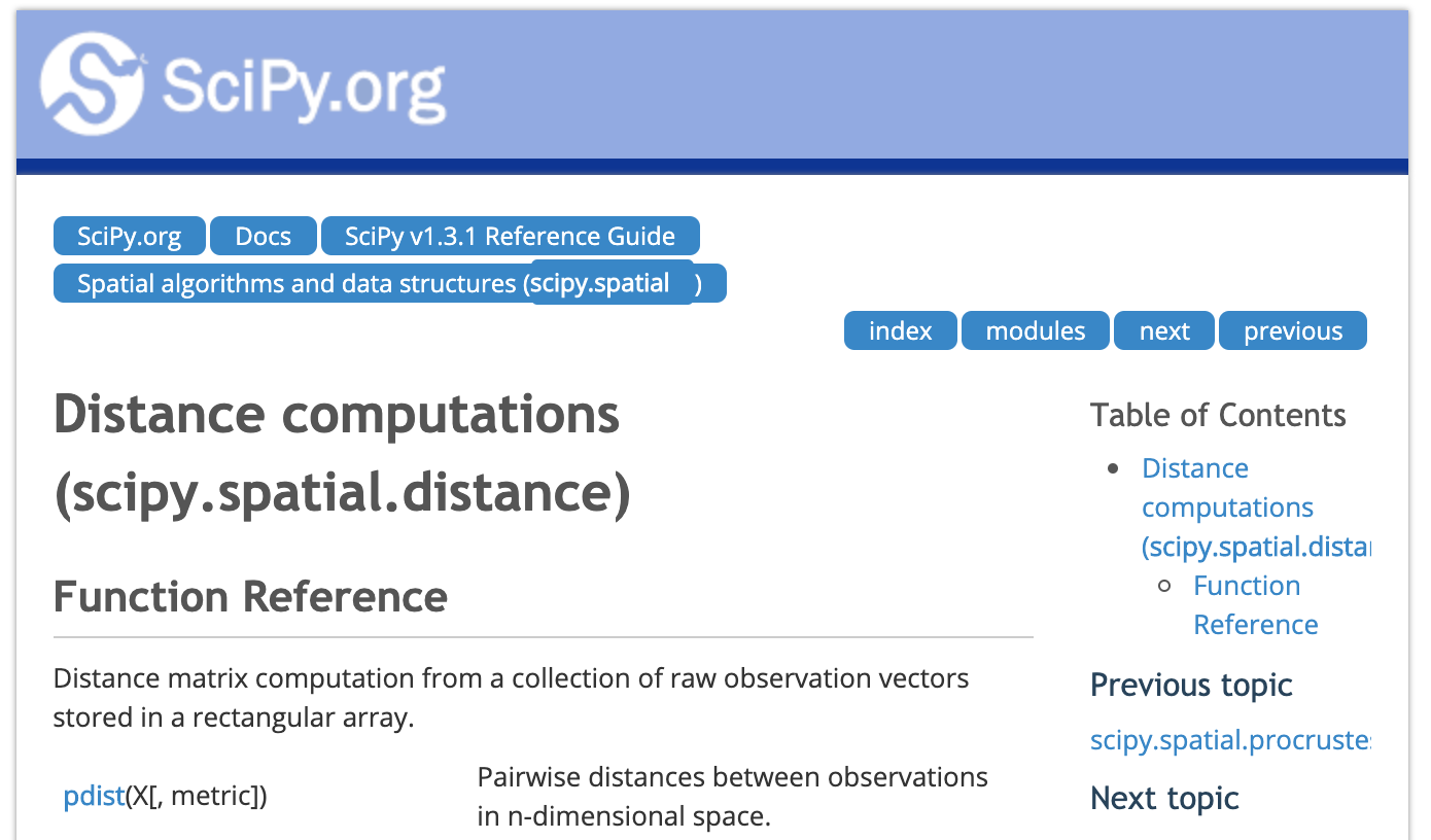
import scipy as sp
sp.spatial.distance.pdist(X) # the pairwise distance: returns (N**2 - N )/2 values for N objects
sp.spatial.distance.squareform(sp.spatial.distance.pdist(wines[["Alcohol", "Magnesium"]]))
#returns the NXN matrix of distances
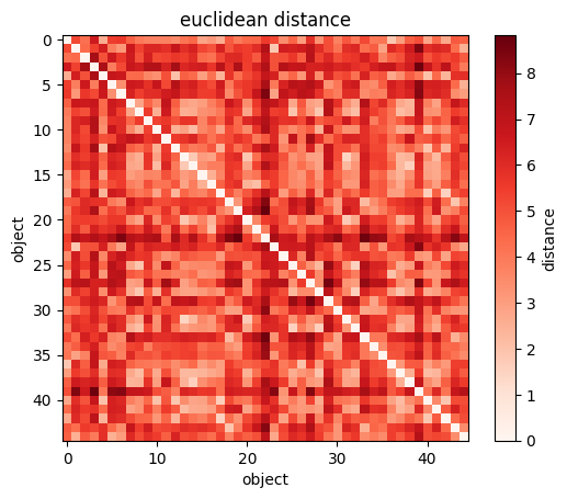
plt.imshow(sp.spatial.distance.squareform(sp.spatial.distance.pdist(wines[["Alcohol", "Magnesium"]])))
#you can visualize the NXN matrix
plt.xlabel("wine")
plt.ylabel("wine");
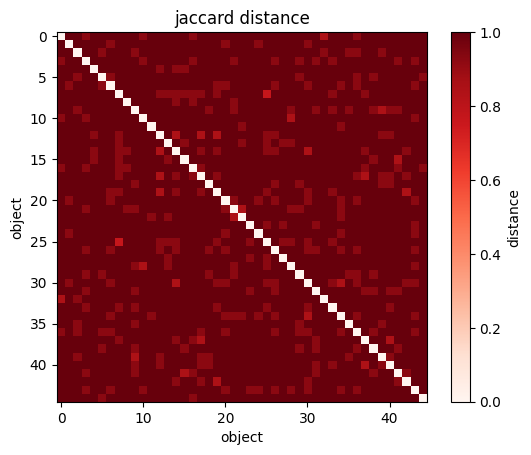
plt.colorbar(label="distance");import scipy as sp
sp.spatial.distance.pdist(X) # the pairwise distance: returns (N**2 - N )/2 values for N objects
sp.spatial.distance.squareform(sp.spatial.distance.pdist(wines[["Alcohol", "Magnesium"]],
metric='jaccard'))
#returns the NXN matrix of distances
plt.imshow(sp.spatial.distance.squareform(sp.spatial.distance.pdist(wines[["Alcohol", "Magnesium"]])))
#you can visualize the NXN matrix
plt.xlabel("wine")
plt.ylabel("wine");
plt.colorbar(label="distance");Minkowski family of distances
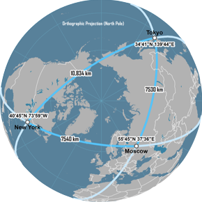
Great Circle distance
features
latitude and longitude
#Great Circle Distance in the sky
import astropy.units as u
from astropy.coordinates import SkyCoord
#The on-sky separation can be computed with the astropy.coordinates.BaseCoordinateFrame.separation()
#or astropy.coordinates.SkyCoord.separation() methods,
#which computes the great-circle distance (not the small-angle approximation):

c1 = SkyCoord('5h23m34.5s', '-69d45m22s', frame='icrs')
c2 = SkyCoord('0h52m44.8s', '-72d49m43s', frame='fk5')
sep = c1.separation(c2)
Angle 20.74611448 deg
from shapely.geometry import Point
import geopandas as gpd
pnt1 = Point(80.99456, 7.86795)
pnt2 = Point(80.97454, 7.872174)
points_df = gpd.GeoDataFrame({'geometry': [pnt1, pnt2]}, crs='EPSG:4326')
points_df = points_df.to_crs('EPSG:5234')
points_df2 = points_df.shift() #We shift the dataframe by 1 to align pnt1 with pnt2
points_df.distance(points_df2)
https://www.codedrome.com/calculating-great-circle-distances-in-python/
https://pypi.org/project/great-circle-calculator/
from math import radians, degrees, sin, cos, asin, acos, sqrt
def great_circle(lon1, lat1, lon2, lat2):
    lon1, lat1, lon2, lat2 = map(radians, [lon1, lat1, lon2, lat2])
    return 6371 * (acos(sin(lat1) * sin(lat2) + cos(lat1) *
cos(lat2) * cos(lon1 - lon2))) #kmUses presence/absence of features in data
: number of features in neither
: number of features in both
: number of features in i but not j
: number of features in j but not i
What is the distance between a leopard and a lizard?
- they both have tails
- only lizards have scales
- neither have wings
Uses presence/absence of features in data
: number of features in neither
: number of features in both
: number of features in i but not j
: number of features in j but not i
What is the distance between a leopard and a lizard?
- they both have tails
- only lizards have scales
- neither have wings
| 1 | 0 | sum | |
|---|---|---|---|
| 1 | M11 | M10 | M11+M10 |
| 0 | M01 | M00 | M01+M00 |
| sum | M11+M01 | M10+M00 | M11+M00+M01+ M10 |
observation i
}
}
| 0 | sum | ||
|---|---|---|---|
| 1 | M10 | M11+M10 | |
| 0 | M01 | M00 | M01+M00 |
| sum | M11+M01 | M10+M00 | M11+M00+M01+ M10 |
1
1
1
0
observation j
Uses presence/absence of features in data
: number of features in neither
: number of features in both
: number of features in i but not j
: number of features in j but not i
What is the distance between a leopard and a lizard?
- they both have tails
- only lizards have scales
- neither have wings
| 1 | 0 | sum | |
|---|---|---|---|
| 1 | M11 | M10 | M11+M10 |
| 0 | M01 | M00 | M01+M00 |
| sum | M11+M01 | M10+M00 | M11+M00+M01+ M10 |
observation i
}
}
| 0 | sum | ||
|---|---|---|---|
| 1 | M10 | M11+M10 | |
| 0 | M01 | M00 | M01+M00 |
| sum | M11+M01 | M10+M00 | M11+M00+M01+ M10 |
observation j
Simple Matching Distance
Uses presence/absence of features in data
: number of features in neither
: number of features in both
: number of features in i but not j
: number of features in j but not i
Simple Matching Coefficient
or Rand similarity
| 1 | 0 | sum | |
|---|---|---|---|
| 1 | M11 | M10 | M11+M10 |
| 0 | M01 | M00 | M01+M00 |
| sum | M11+M01 | M10+M00 | M11+M00+M01+ M10 |
observation i
observation j
}
}
| 0 | sum | ||
|---|---|---|---|
| 1 | M11 | M10 | M11+M10 |
| 0 | M01 | M00 | M01+M00 |
| sum | M11+M01 | M10+M00 | M11+M00+M01+ M10 |
lizard/leopard
1
1
1
0
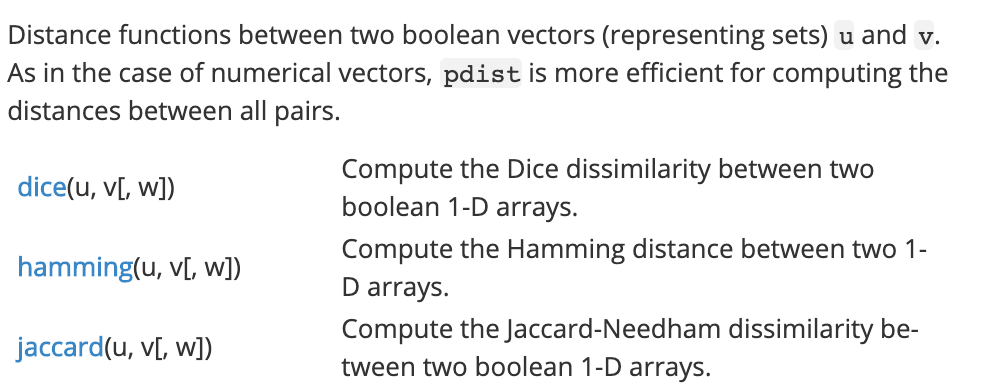
Jaccard similarity
Jaccard distance
| 1 | 0 | sum | |
|---|---|---|---|
| 1 | M11 | M10 | M11+M10 |
| 0 | M01 | M00 | M01+M00 |
| sum | M11+M01 | M10+M00 | M11+M00+M01+ M10 |
observation i
observation j
}
}
lizard/leopard
Jaccard similarity
Jaccard distance
| 1 | 0 | sum | |
|---|---|---|---|
| 1 | M11 | M10 | M11+M10 |
| 0 | M01 | M00 | M01+M00 |
| sum | M11+M01 | M10+M00 | M11+M00+M01+ M10 |
observation i
observation j
}
}
Jaccard similarity
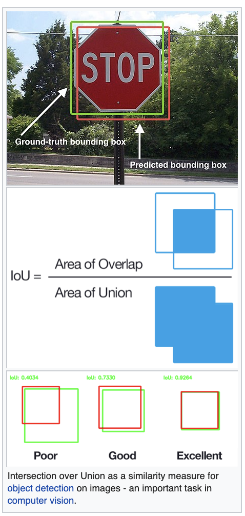
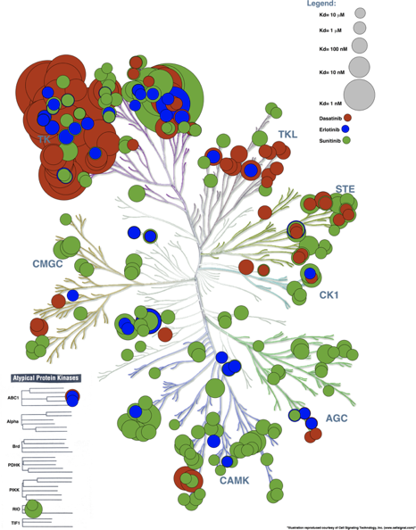
Application to Deep Learning for image recognition
Convolutional Neural Nets
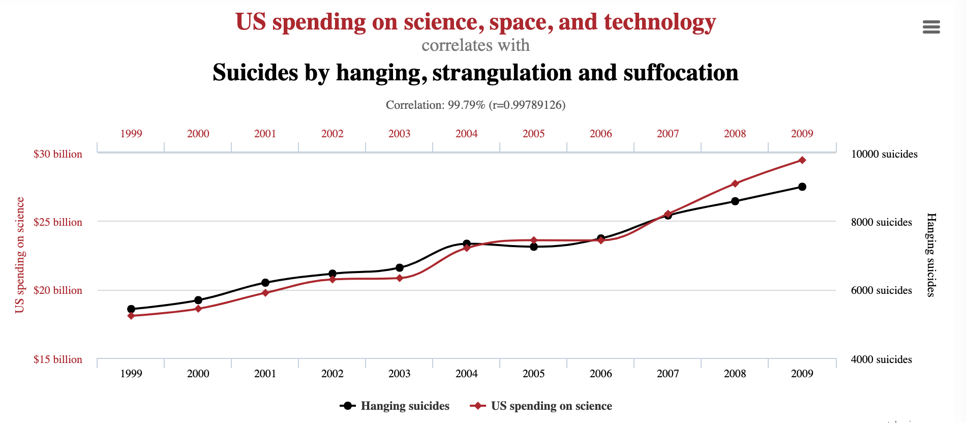
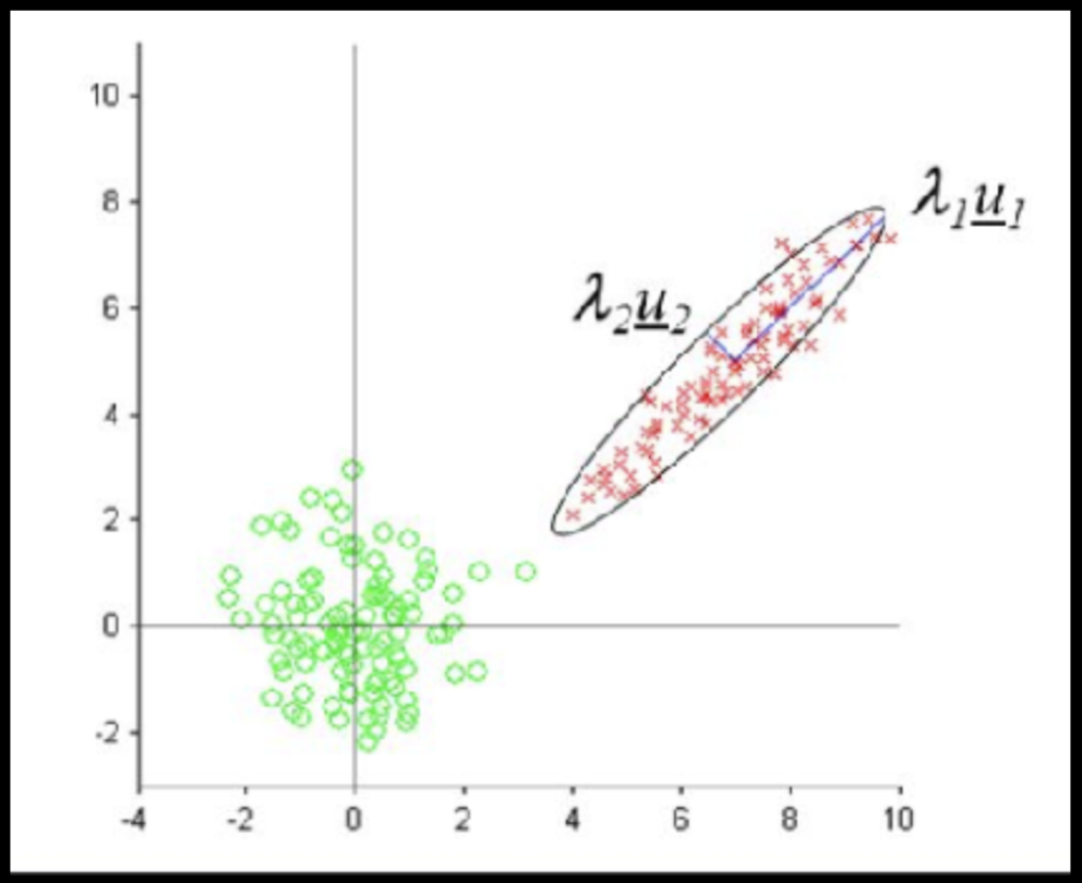
Data can have covariance (and it almost always does!)
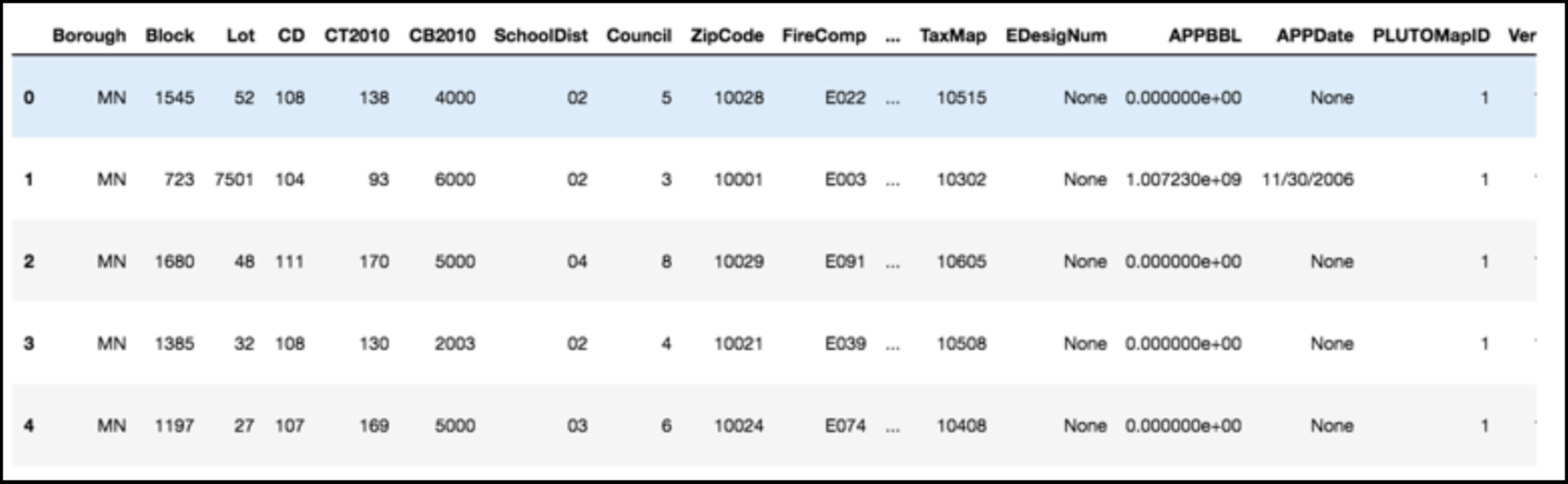
PLUTO Manhattan data (42,000 x 15)
axis 1 -> features
axis 0 -> observations
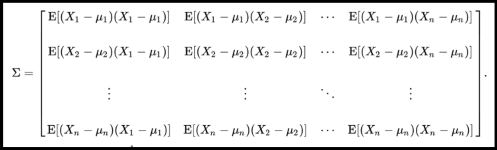
Data can have covariance (and it almost always does!)
Data can have covariance (and it almost always does!)
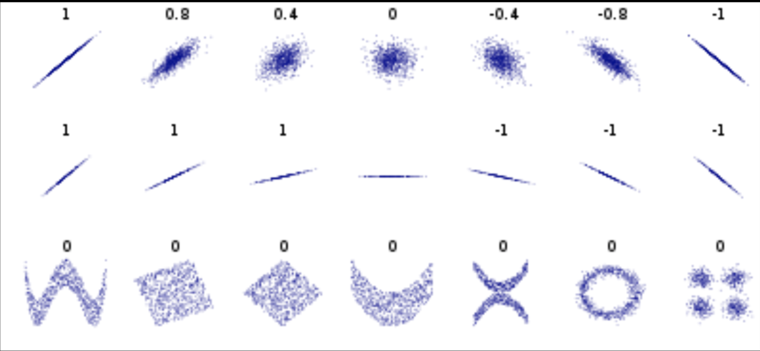
Pearson's correlation (linear correlation)
correlation = correlation / variance
PLUTO Manhattan data (42,000 x 15) correlation matrix
axis 1 -> features
axis 0 -> observations
Data can have covariance (and it almost always does!)
PLUTO Manhattan data (42,000 x 15) correlation matrix
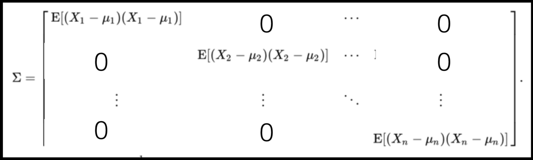
A covariance matrix is diagonal if the data has no correlation
Data can have covariance (and it almost always does!)
Full On Whitening
find the matrix W that diagonalized Σ
from zca import ZCA
import numpy as np
X = np.random.random((10000, 15)) # data array
trf = ZCA().fit(X)
X_whitened = trf.transform(X)
X_reconstructed =
trf.inverse_transform(X_whitened)
assert(np.allclose(X, X_reconstructed))
: remove covariance by diagonalizing the transforming the data with a matrix that diagonalizes the covariance matrix
this is at best hard, in some cases impossible even numerically on large datasets
Data that is not correlated appear as a sphere in the Ndimensional feature space
Data can have covariance (and it almost always does!)
ORIGINAL DATA
STANDARDIZED DATA
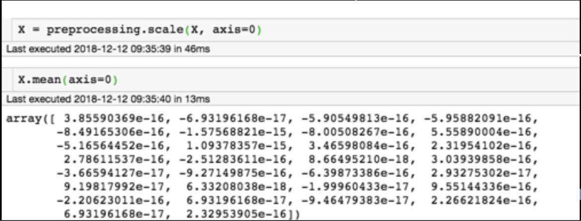
Generic preprocessing
Generic preprocessing
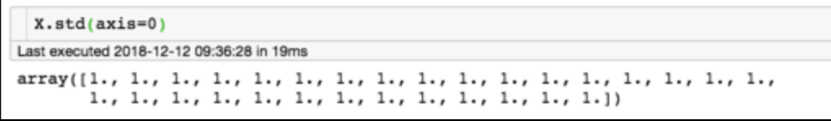
for each feature: divide by standard deviation and subtract mean
mean of each feature should be 0, standard deviation of each feature should be 1
K-means (McQueen ’67)
K-medoids (Kaufman & Rausseeuw ’87)
Expectation Maximization (Dempster,Laird,Rubin ’77)
Hard partitioning cluster method
Choose N “centers” guesses: random points in the feature space
repeat:
  Calculate distance between each point and each center

  Assign each point to the closest center

  Calculate the new cluster centers

untill (convergence):
  when clusters no longer change
Objective: minimizing the aggregate distance within the cluster.
Order: #clusters #dimensions #iterations #datapoints O(KdN)
CONs:
Its non-deterministic: the result depends on the (random) starting point
It only works where the mean is defined: alternative is K-medoids which represents the cluster by its central member (median), rather than by the mean
Must declare the number of clusters upfront (how would you know it?)
PROs:
Scales linearly with d and N
Objective: minimizing the aggregate distance within the cluster.
Order: #clusters #dimensions #iterations #datapoints O(KdN)
O(KdN):
complexity scales linearly with
-d number of dimensions
-N number of datapoints
-K number of clusters
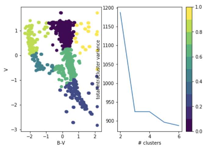
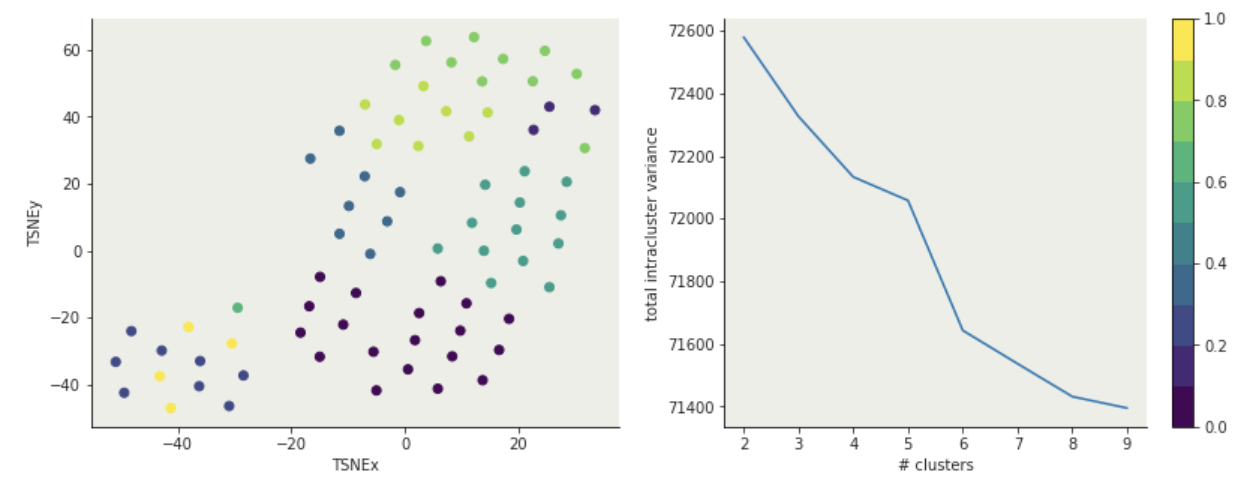
either you know it because of domain knowledge
or
you choose it after the fact: "elbow method"
total intra-cluster variance
Objective: minimizing the aggregate distance within the cluster.
Order: #clusters #dimensions #iterations #datapoints O(KdN)
Must declare the number of clusters
Objective: minimizing the aggregate distance within the cluster.
Order: #clusters #dimensions #iterations #datapoints O(KdN)
Must declare the number of clusters upfront (how would you know it?)
either domain knowledge or
after the fact: "elbow method"
total intra-cluster variance
‘k-means++’ : selects initial cluster centers for k-mean clustering in a smart way to speed up convergence. See section Notes in k_init for more details.
‘random’: choose k observations (rows) at random from data for the initial centroids.
If an ndarray is passed, it should be of shape (n_clusters, n_features) and gives the initial centers.
Soft partitioning cluster method
Hard clustering : each object in the sample belongs to only 1 cluster
Soft clustering : to each object in the sample we assign a degree of belief that it belongs to a cluster
Soft = probabilistic
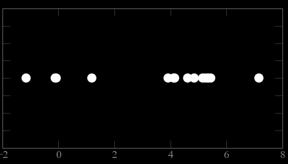
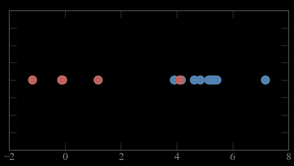
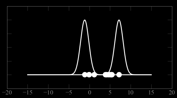
these points come from 2 gaussian distribution.
which point comes from which gaussian?
1
2
3
4-6
7
8
9-12
13
CASE 1:
if i know which point comes from which gaussian
i can solve for the parameters of the gaussian
(e.g. maximizing likelihood)
1
2
3
4-6
7
8
9-12
13
CASE 2:
if i know which the parameters (μ,σ) of the gaussians
i can figure out which gaussian each point is most likely to come from (calculate probability)
1
2
3
4-6
7
8
9-12
13
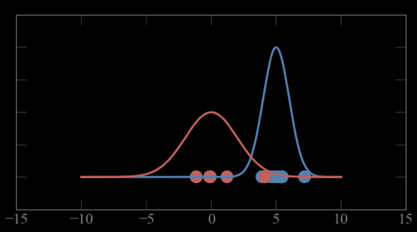
Guess parameters g= (μ,σ) for 2 Gaussian distributions A and B
calculate the probability of each point to belong to A and B
Guess parameters g= (μ,σ) for 2 Gaussian distributions A and B
calculate the probability of each point to belong to A and B
high
low
Guess parameters g= (μ,σ) for 2 Gaussian distributions A and B
calculate the probability of each point to belong to A and B
Guess parameters g= (μ,σ) for 2 Gaussian distributions A and B
1- calculate the probability p_ji of each point to belong to gaussian j
Bayes theorem: P(A|B) = P(B|A) P(A) / P(B)
Guess parameters g= (μ,σ) for 2 Gaussian distributions A and B
1- calculate the probability p_ji of each point to belong to gaussian j
2a - calculate the weighted mean of the cluster, weighted by the p_ji
Bayes theorem: P(A|B) = P(B|A) P(A) / P(B)
Bayes theorem: P(A|B) = P(B|A) P(A) / P(B)
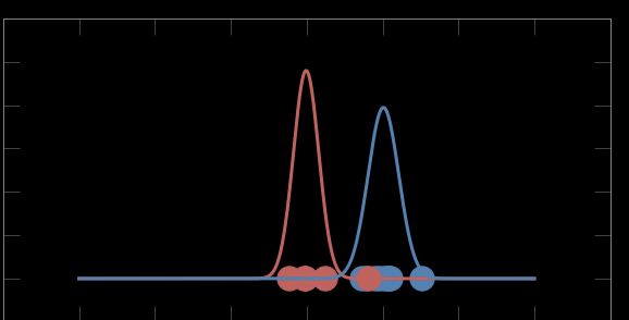
Guess parameters g= (μ,σ) for 2 Gaussian distributions A and B
1- calculate the probability p_ji of each point to belong to gaussian j
2a - calculate the weighted mean of the cluster, weighted by the p_ji
2b - calculate the weighted sigma of the cluster, weighted by the p_ji
Bayes theorem: P(A|B) = P(B|A) P(A) / P(B)
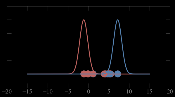
Alternate expectation and maximization step till convergence
1- calculate the probability p_ji of each point to belong to gaussian j
2a - calculate the weighted mean of the cluster, weighted by the p_ji
2b - calculate the weighted sigma of the cluster, weighted by the p_ji
expectation step
maximization step
}
Last iteration: convergence
Bayes theorem: P(A|B) = P(B|A) P(A) / P(B)
Alternate expectation and maximization step till convergence
1- calculate the probability p_ji of each point to belong to gaussian j
2a - calculate the weighted mean of the cluster, weighted by the p_ji
2b - calculate the weighted sigma of the cluster, weighted by the p_ji
expectation step
maximization step
}
Choose N “centers” guesses (like in K-means)
repeat
Expectation step: Calculate the probability of each distribution given the points

Maximization step: Calculate the new centers and variances as weighted averages of the datapoints, weighted by the probabilities
untill (convergence)
e.g. when gaussian parameters no longer change
Order: #clusters #dimensions #iterations #datapoints #parameters O(KdNp) (>K-means)
based on Bayes theorem
Its non-deterministic: the result depends on the (random) starting point (like K-mean)
It only works where a probability distribution for the data points can be defines (or equivalently a likelihood) (like K-mean)
Must declare the number of clusters and the shape of the pdf upfront (like K-mean)
Convergence Criteria
General
Any time you have an objective function (or loss function) you need to set up a tolerance : if your objective function did not change by more than ε since the last step you have reached convergence (i.e. you are satisfied)
ε is your tolerance
For clustering:
convergence can be reached if
no more than n data point changed cluster
n is your tolerance
dataset
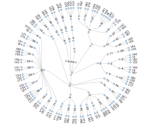
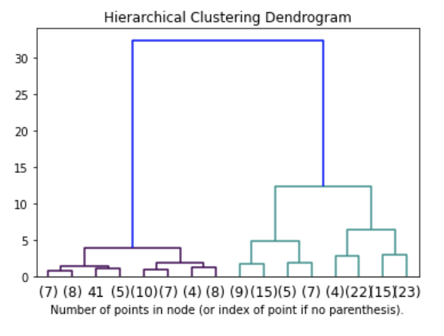
Cluster Visualization "dendrogram"
distance
it's deterministic!
it's deterministic!
computationally intense because every cluster pair distance has to be calculate
it's deterministic!
computationally intense because every cluster pair distance has to be calculate
it is slow, though it can be optimize:
complexity
compute the distance matrix
each data point is a singleton cluster
repeat
    merge the 2 cluster with minimum distance
    update the distance matrix
untill
    only a single (n) cluster(s) remains
Order:
PROs
It's deterministic
CONs
It's greedy (optimization is done step by step and agglomeration decisions cannot be undone)
It's computationally expensive
distance between a point and a cluster:
single link distance
D(c1,c2) = min(D(xc1, xc2))
distance between a point and a cluster:
single link distance
D(c1,c2) = min(D(xc1, xc2))
complete link distance
D(c1,c2) = max(D(xc1, xc2))
distance between a point and a cluster:
single link distance
D(c1,c2) = min(D(xc1, xc2))
complete link distance
D(c1,c2) = max(D(xc1, xc2))
centroid link distance
D(c1,c2) = mean(D(xc1, xc2))
distance between a point and a cluster:
single link distance
D(c1,c2) = min(D(xc1, xc2))
complete link distance
D(c1,c2) = max(D(xc1, xc2))
centroid link distance
D(c1,c2) = mean(D(xc1, xc2))
Ward distance (global measure)
it is
non-deterministic
(like k-mean)
it is
non-deterministic
(like k-mean)
it is greedy -
just as k-means
two nearby points
may end up in
separate clusters
it is
non-deterministic
(like k-mean)
it is greedy -
just as k-means
two nearby points
may end up in
separate clusters
it is high complexity for
exhaustive search
But can be reduced (~k-means)
or
Calculate clustering criterion for all subgroups, e.g. min intracluster variance
repeat
split the best cluster based on criterion above
untill
each data is in its own singleton cluster
Order: (w K-means procedure)
It's non-deterministic: the result depends on the (random) starting point (like K-mean) unless its exaustive (but that is )
or
It's greedy (optimization is done step by step)
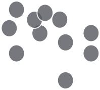
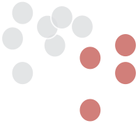
DBSCAN
DBSCAN is one of the most common clustering algorithms and also most cited in scientific literature
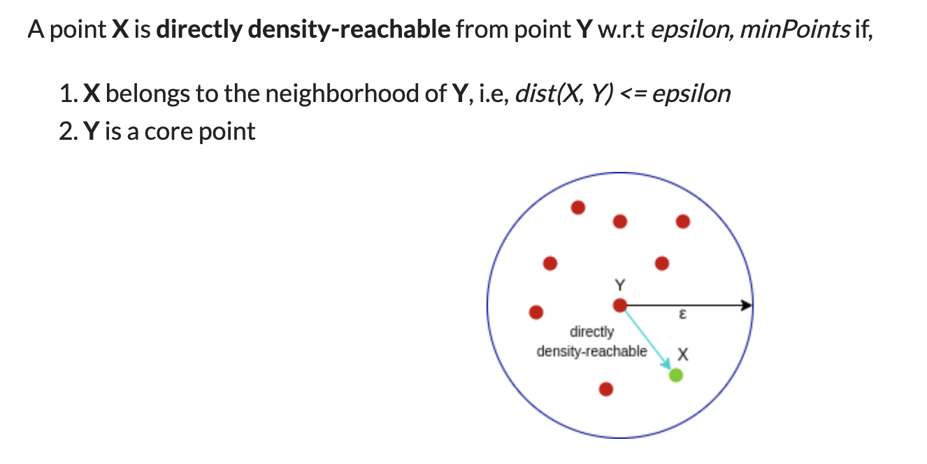
A point p is a core point if at least minPts points are within distance ε (including p).
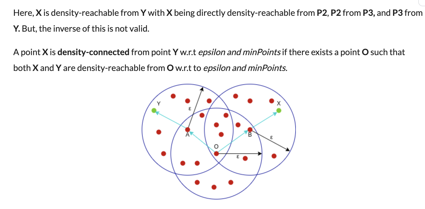
A point q is directly reachable from p if point q is within distance ε from core point p. Reachable from p if there is a path p1, ..., pn with p1 = p and pn = q, where each pi+1 is directly reachable from pi.
All points not reachable from any other point are outliers or noise points.
Density-based spatial clustering of applications with noise
minPts
minimum number of points to form a dense region
maximum distance for points to be considered part of a cluster
ε
Key Hyperparameters:
Density-based spatial clustering of applications with noise
Key Hyperparameters:
minPts
minimum number of points to form a dense region
ε
maximum distance for points to be considered part of a cluster
2 points are considered neighbors if distance between them <= ε
Density-based spatial clustering of applications with noise
minPts
ε
maximum distance for points to be considered part of a cluster
minimum number of points to form a dense region
2 points are considered neighbors if distance between them <= ε
regions with number of points >= minPts are considered dense
Key Hyperparameters:
ε
minPts = 3
slides: Farid Qmar
ε
minPts = 3
slides: Farid Qmar
ε
minPts = 3
ε
slides: Farid Qmar
ε
minPts = 3
directly reachable
slides: Farid Qmar
ε
minPts = 3
core
dense region
slides: Farid Qmar
ε
minPts = 3
slides: Farid Qmar
ε
minPts = 3
directly reachable to
slides: Farid Qmar
ε
minPts = 3
reachable to
slides: Farid Qmar
ε
minPts = 3
slides: Farid Qmar
ε
minPts = 3
reachable
slides: Farid Qmar
ε
minPts = 3
slides: Farid Qmar
ε
minPts = 3
slides: Farid Qmar
ε
minPts = 3
ε
slides: Farid Qmar
ε
minPts = 3
directly reachable
slides: Farid Qmar
ε
minPts = 3
core
dense region
slides: Farid Qmar
ε
minPts = 3
reachable
slides: Farid Qmar
ε
minPts = 3
slides: Farid Qmar
ε
minPts = 3
noise/outliers
slides: Farid Qmar
PROs:
CONs:
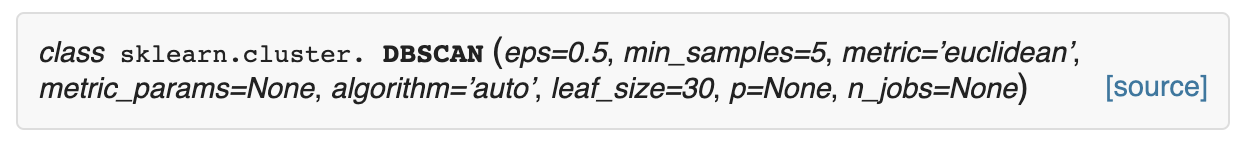
ε : minimum distance to join points
min_sample : minimum number of points in a cluster, otherwise they are labeled outliers.
metric : the distance metric
p : float, optional The power of the Minkowski metric
ε : minimum distance to join points
min_sample : minimum number of points in a cluster, otherwise they are labeled outliers.
metric : the distance metric
p : float, optional The power of the Minkowski metric
its extremely sensitive to these parameters!
for each point P count neighbours within minPts: label=C
for each point P ~= C measure distance d to all Cs
        if d<minD: label = DR
for each point P not C and not DR
        if distance d to C or DR > minD: label = outlier
        if distance d to C or DR <= minD: find path to closet C and cluster
Order:
PROs
Deterministic.
Deals with noise and outliers
Can be used with any definition of distance or similarity
PROs
Not entirely deterministic.
Only works in a constant density field
a really good blog post on DBScan
https://www.analyticsvidhya.com/blog/2020/09/how-dbscan-clustering-works/
Clustering : unsupervised learning where all features are observed for all datapoints. The goal is to partition the space into maximally homogeneous maximally distinguished groups
clustering is easy, but interpreting results is tricky
Distance : A definition of distance is required to group observations/ partition the space.
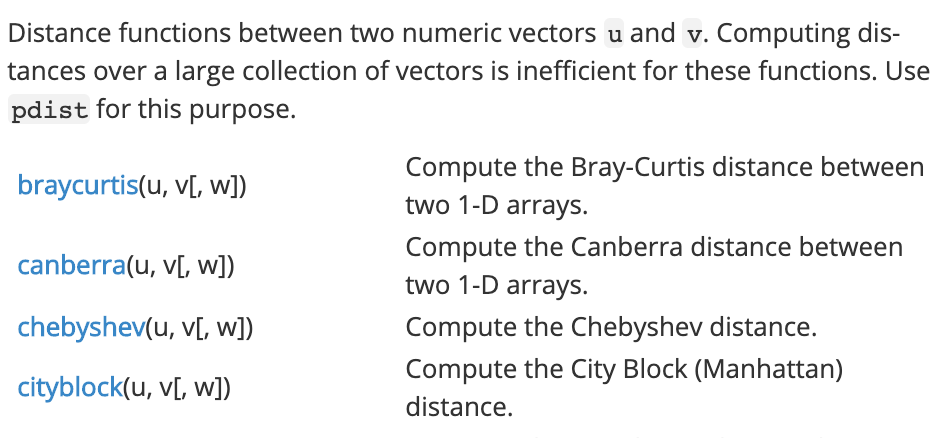
Common distances over continuous variables
Common distances over categorical variables:
Whitening
Models assume that the data is not correlated. If your data is correlated the model results may be invalid. And your data always has correlations.
- whiten the data by using the matrix that diagonalizes the covariance matrix. This is ideal but computationally expensive if possible at all
- scale your data so that each feature is mean=0 stdev=2.
Solution:
Partition clustering:
Hard: K-means O(KdN) , needs to decide the number of clusters, non deterministic
simple efficient implementation but the need to select the number of clusters is a significant flaw
Soft: Expectation Maximization O(KdNp) , needs to decide the number of clusters, need to decide a likelihood function (parametric), non deterministic
Hierarchical:
Divisive: Exhaustive ; at least non deterministic
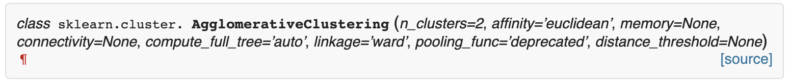
Agglomerative: , deterministic, greedy. Can be run through and explore the best stopping point. Does not require to choose the number of clusters a priori
Density based
DBSCAN: Density based clustering method that can identify outliers, which means it can be used in the presence of noise. Complexity . Most common (cited) clustering method in the natural sciences.
encoding categorical variables:
variables have to be encoded as numbers for computers to understand them. You can encode categorical variables with integers or floating point but you implicitly impart an order. The standard is to one-hot-encode which means creating a binary (True/False) feature (column) for each category of a categorical variables but this increases the feature space and generated covariance.
model diagnostics for classifiers: Fraction of True Positives and False Positives are the metrics to evaluate classifiers. Combinations of those numbers include Accuracy (TP/ (TP+FP)), Precision (TP/(TP+FN)), Recall ((TP+TN)/(TP+TN+FP+FN)).
ROC curve: (TP vs FP) is a holistic metric of a model. It can be used to guide the choice of hyperparameters to find the "sweet spot" for your problem
a comprehensive review of clustering methods
Data Clustering: A Review, Jain, Mutry, Flynn 1999
https://www.cs.rutgers.edu/~mlittman/courses/lightai03/jain99data.pdf
a blog post on how to generate and interpret a scipy dendrogram by Jörn Hees
https://joernhees.de/blog/2015/08/26/scipy-hierarchical-clustering-and-dendrogram-tutorial/
Any of these papers:
By federica bianco
clustering


