


federica bianco PRO
astro | data science | data for good
2023
University of Delaware
Department of Physics and Astronomy
federica bianco
Biden School of Public Policy and Administration
Data Science Institute
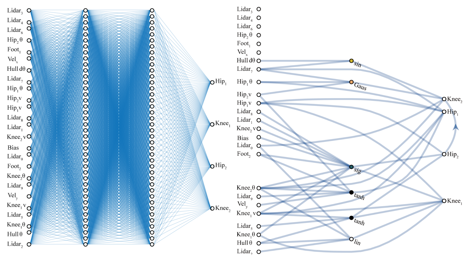
Li et al. 2022
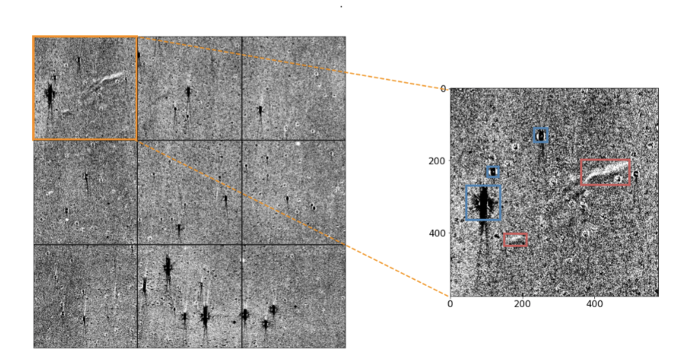
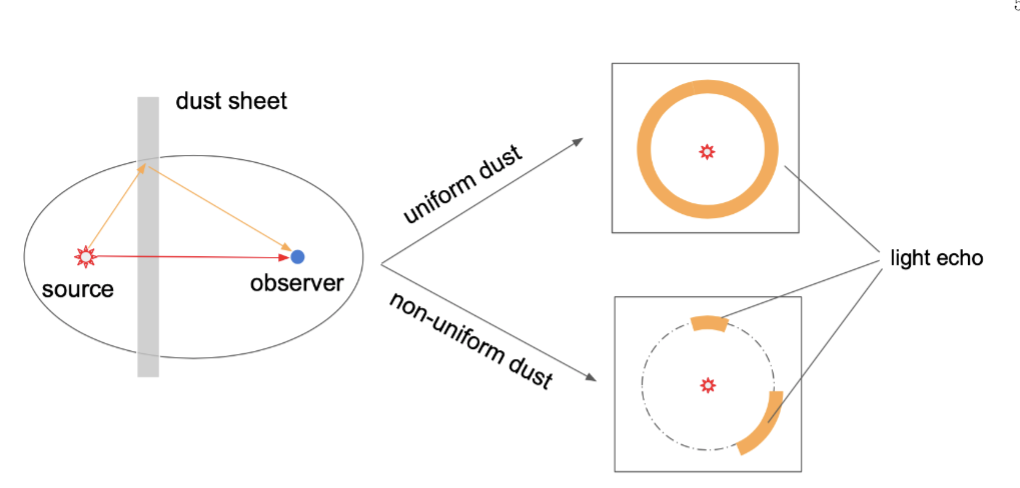
AILE: the first AI-based platform for the detection and study of Light Echoes
NSF Award #2108841
Pessimal AI problem:
Xiaolong Li
LSSTC Catalyst Fellow 2023
UDelaware->John Hopkins
AILE: the first AI-based platform for the detection and study of Light Echoes
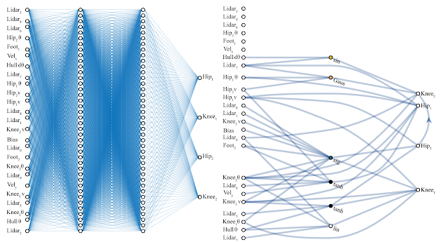
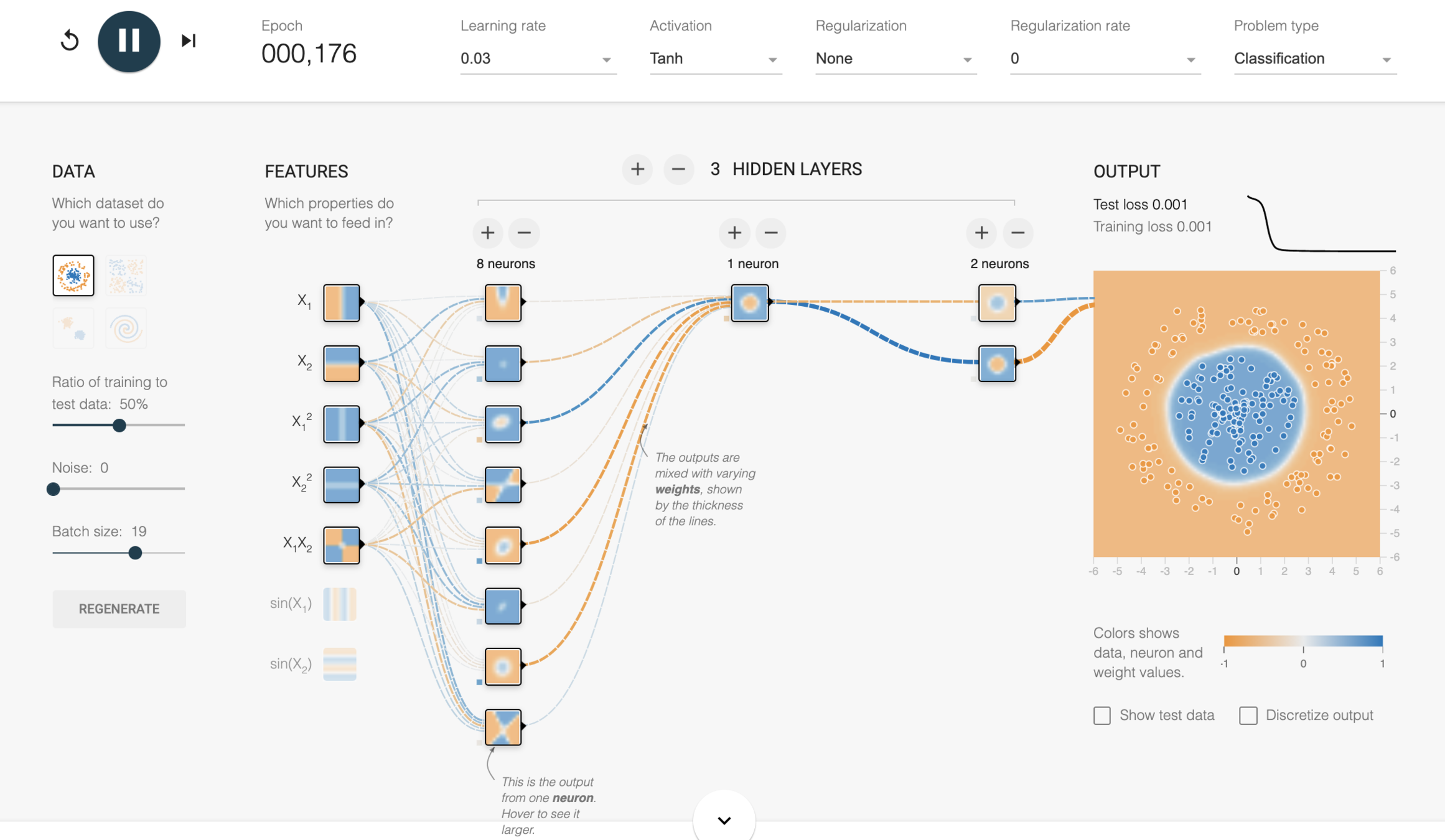
YOLO3 + "attention" mechanism
precision 80% at 70% recall with a training set of 19 light echo examples!
Xiaolong Li
LSSTC Catalyst Fellow 2023
UDelaware->John Hopkins
Time ->
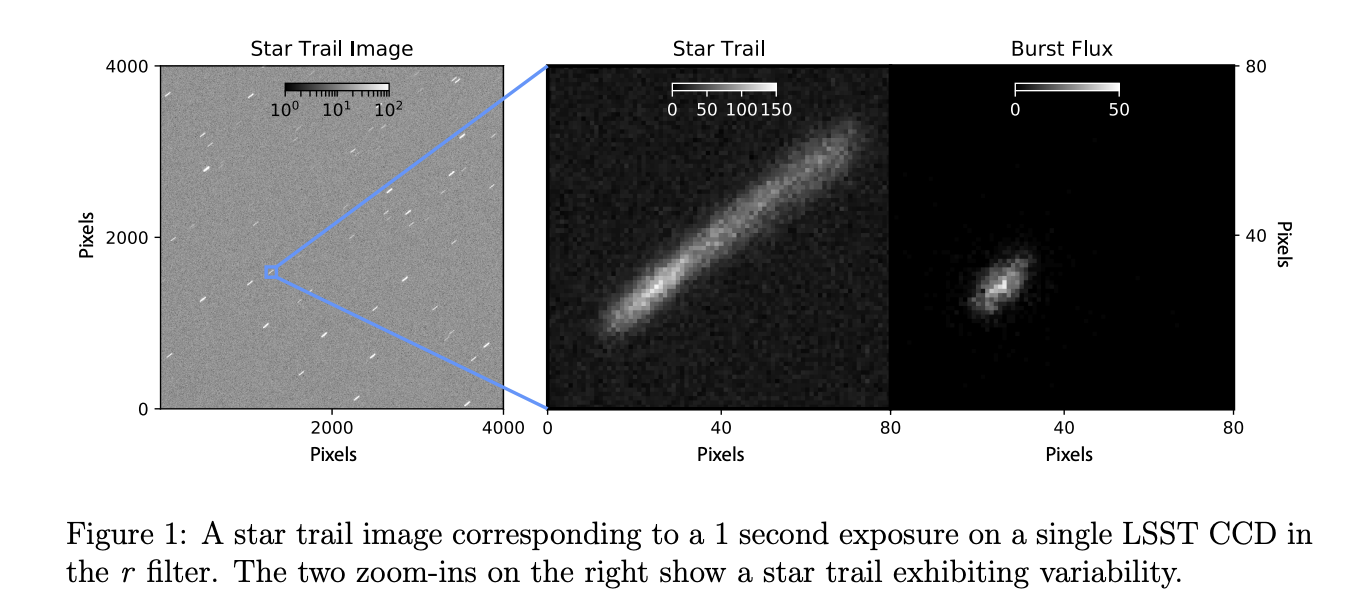
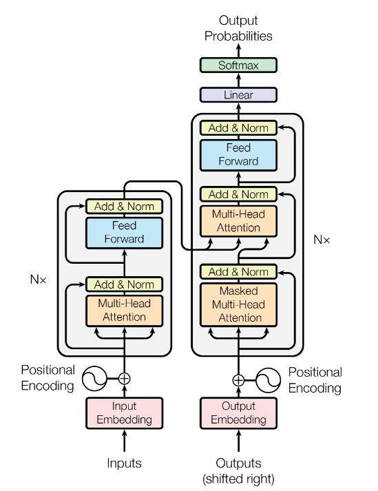
Language models for time-resolved image processing
Shar Daniels
UDel 1st year
ZTF time-resolved continuous readout images (w Igor Andreoni and Ashish Mahabal)
Transformer architecture
NN for language processing
Educate Policy makers
without understanding how ML works policy makers do not have the instruments to regulate it
Education for the people
but does this put the burden on the victims?
Educating DS practitioners in communicating DS concepts
the put the burden back on the practitioners
Datascience Education to Help and Protect us
Jack Dorsey (Twitter CEO) at TED 2019
boring the TED audience with details
Zuckerberg (Facebook CEO) deflecting questions at senate hearing
used to:
Inferential AI
Generative AI
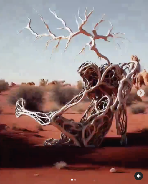
Generative AI
https://www.instagram.com/p/CtO_80PM6BD/
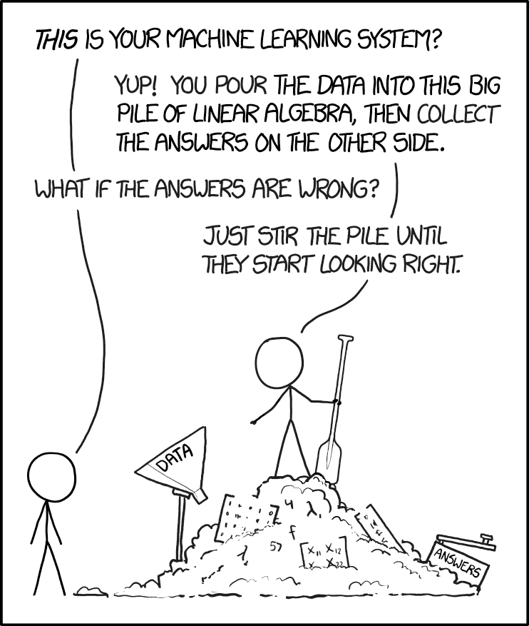
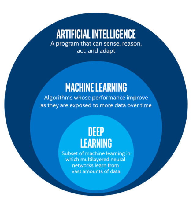
[Machine Learning is the] field of study that gives computers the ability to learn without being explicitly programmed.
Arthur Samuel, 1959
what is a ML?
a model is a low dimensional representation of a higher dimensionality datase
what is a "model" in ML?
Any mathematical model with parameters that are
learned from the data
what is a ML "model"?
what is a ML "model"?
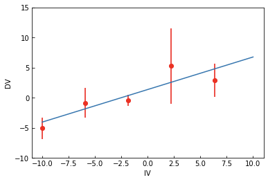
mathematical formula: y = ?
model parameters: slope a, intercept b
mathematical formula: y = ax + b
what is a ML "model"?
model parameters: slope a, intercept b
mathematical formula: y = ax + b
what is a ML "model"?
ML: study, development, and applicaton of any model with parameters learnt from the data
time
time
time
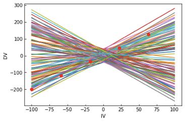
which is the "best fit" line? A , B, C, D?
A
B
C
D
x1
x2
Machine Learning models are parametrized representation of "reality" where the parameters are learned from finite sets of realizations of that reality
(note: learning by instance, e.g. nearest neighbours, may not comply to this definition)
Machine Learning is the disciplines that conceptualizes, studies, and applies those models.
Key Concept
what is machine learning?
model parameters are learned by calculating a loss function for diferent parameter sets and trying to minimize loss (or a target function and trying to maximize)
e.g.
L1 = |target - prediction|
Learning relies on the definition of a loss function
Machine Learning
Data driven models for exploration of structure
set up: All features known for all observations
Goal: explore structure in the data
- data compression
- understanding structure
Algorithms: Clustering, (...)
x
y
Unsupervised Learning
Data driven models for exploration of structure
Unsupervised Learning
| learning type | loss / target |
|---|---|
| unsupervised | intra-cluster variance / inter cluster distance |
Data driven models for prediction
set up: All features known for a sunbset of the data; one feature cannot be observed for the rest of the data
Goal: predicting missing feature
- classification
- regression
Algorithms: regression, SVM, tree methods, k-nearest neighbors, neural networks, (...)
x
y
Supervised Learning
Learning relies on the definition of a loss function
| learning type | loss / target |
|---|---|
| unsupervised | intra-cluster variance / inter cluster distance |
| supervised | distance between prediction and truth |
Machine Learning
Some FREE references!
michael nielsen
better pedagogical approach, more basic, more clear
ian goodfellow
mathematical approach, more advanced, unfinished
michael nielsen
better pedagogical approach, more basic, more clear
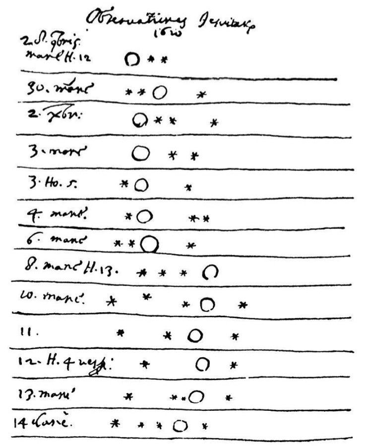
Galileo Galilei 1610
Following: Djorgovski
https://events.asiaa.sinica.edu.tw/school/20170904/talk/djorgovski1.pdf
Experiment driven
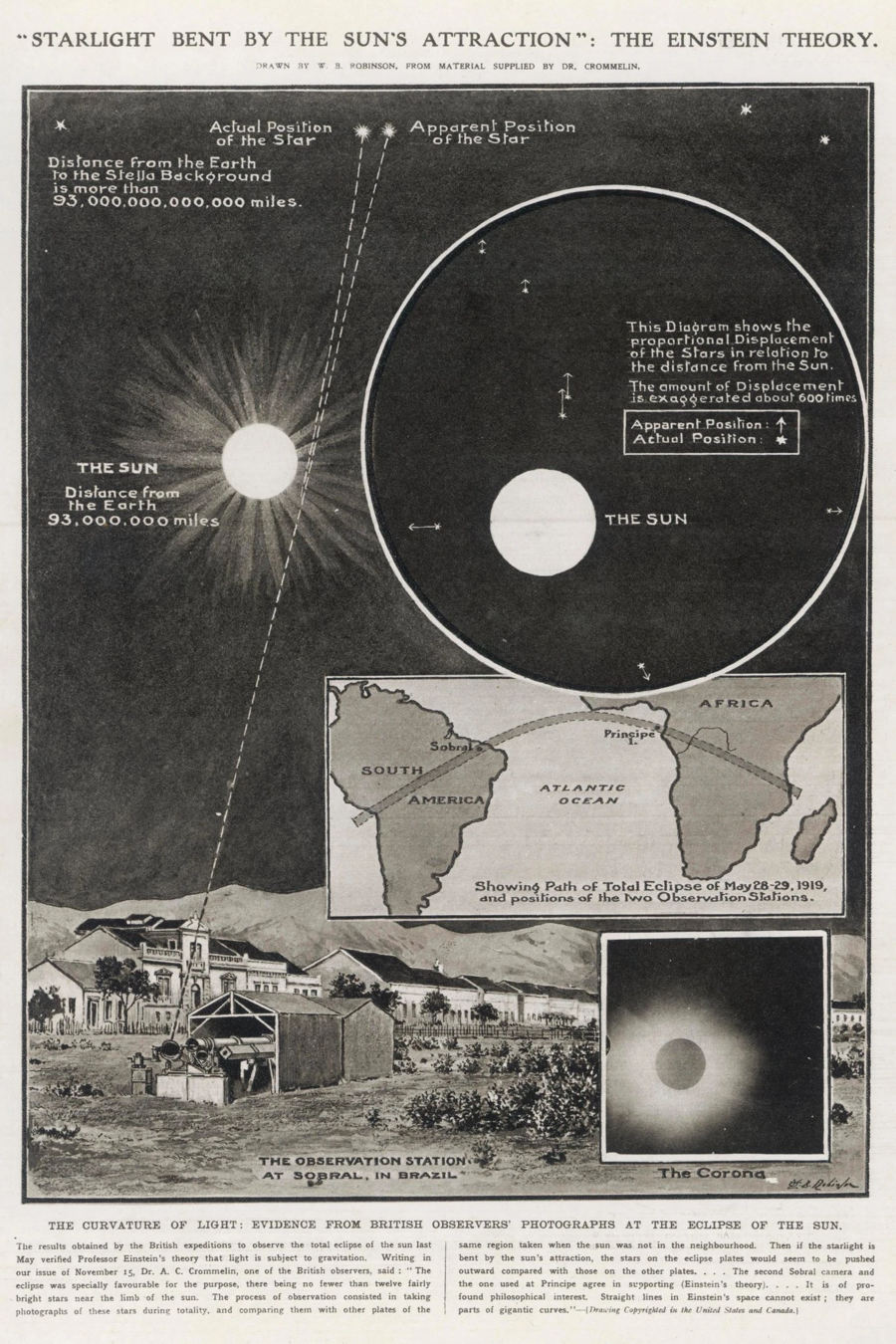
Enistein 1916
Theory driven | Falsifiability
Experiment driven
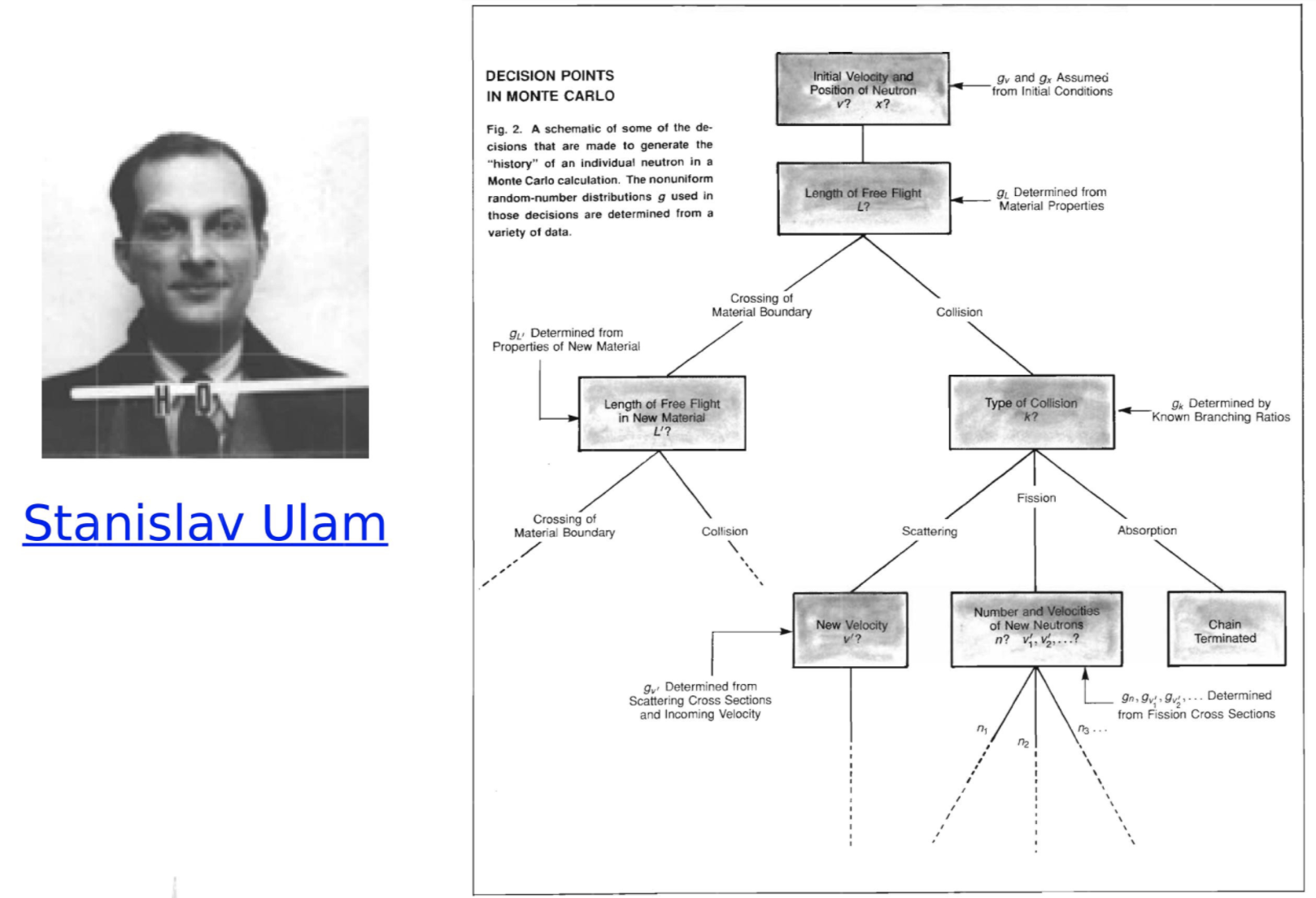
Ulam 1947
Theory driven | Falsifiability
Experiment driven
Simulations | Probabilistic inference | Computation
http://www-star.st-and.ac.uk/~kw25/teaching/mcrt/MC_history_3.pdf
the 2000s
Theory driven | Falsifiability
Experiment driven
Simulations | Probabilistic inference | Computation
Big Data + Computation | pattern discovery | predict by association
data driven: lots of data, drop theory and use associations
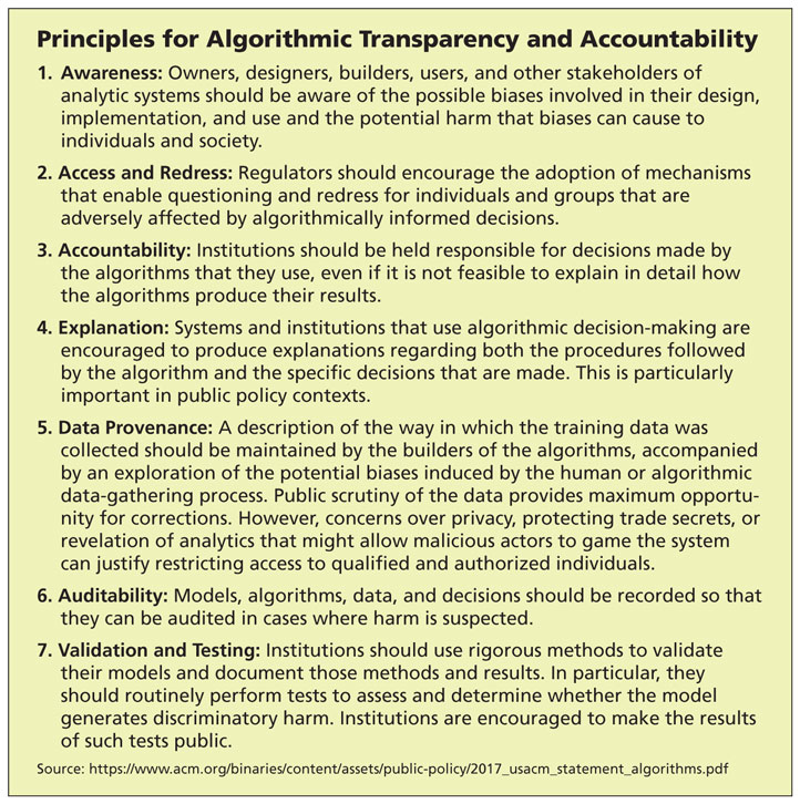
strictly policy issues:
proprietary algorithms + audability
technical + policy issues:
data access and redress + data provenance
https://www.darpa.mil/attachments/XAIProgramUpdate.pdf
trivially intuitive
generalized additive models
decision trees
SVM
Random Forest
Deep Learning
Accuracy
univaraite
linear
regression
we're still trying to figure it out
https://www.darpa.mil/attachments/XAIProgramUpdate.pdf
trivially intuitive
generalized additive models
decision trees
SVM
Random Forest
Deep Learning
Accuracy in solving complex problems
univaraite
linear
regression
we're still trying to figure it out
trivially intuitive
generalized additive models
decision trees
Deep Learning
number of features that can be effectively included in the model
thousands
1
SVM
Random Forest
univaraite
linear
regression
https://www.darpa.mil/attachments/XAIProgramUpdate.pdf
Accuracy in solving complex problems
we're still trying to figure it out
trivially intuitive
univaraite
linear
regression
generalized additive models
decision trees
Deep Learning
SVM
Random Forest
https://www.darpa.mil/attachments/XAIProgramUpdate.pdf
time
Accuracy in solving complex problems
we're still trying to figure it out
1
Machine learning: any method that learns parameters from the data
2
The transparency of an algorithm is proportional to its complexity and the complexity of the data space
3
The transparency of an algorithm is limited by our own ability and preparedness to interpret it
Toward Interpretable Machine Learning, Samek+2003
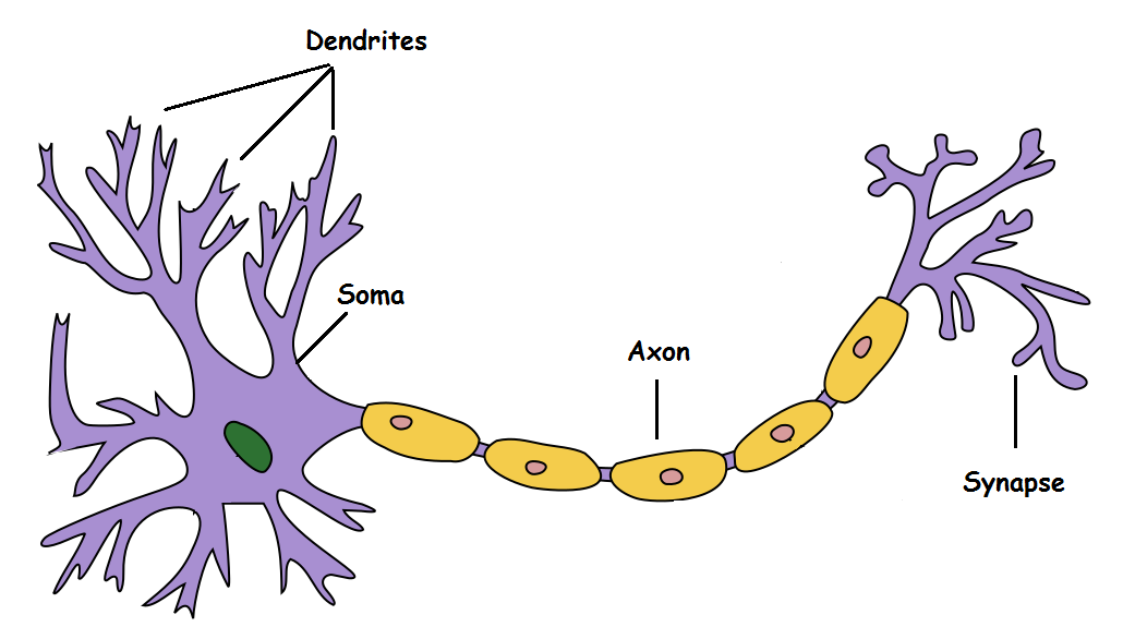
Neural Networks
1
Neural Networks
1.1
origins
1943
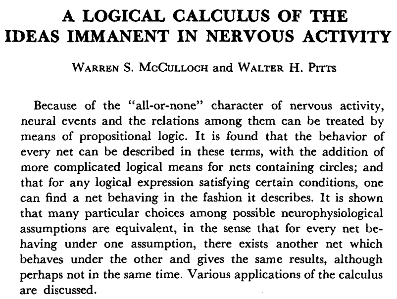
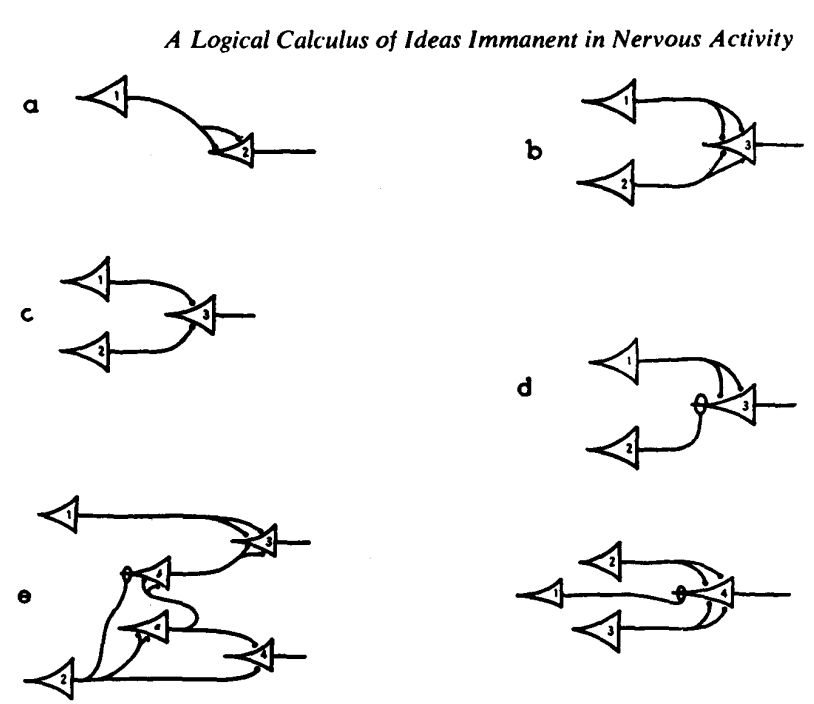
M-P Neuron McCulloch & Pitts 1943
1943
M-P Neuron McCulloch & Pitts 1943
1943
M-P Neuron McCulloch & Pitts 1943
M-P Neuron
1943
M-P Neuron
its a classifier
M-P Neuron McCulloch & Pitts 1943
M-P Neuron
1943
M-P Neuron McCulloch & Pitts 1943
M-P Neuron
1943
if is Bool (True/False)
what value of corresponds to logical AND?
M-P Neuron McCulloch & Pitts 1943
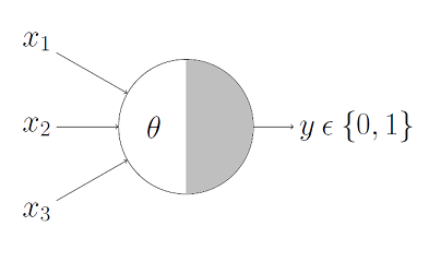
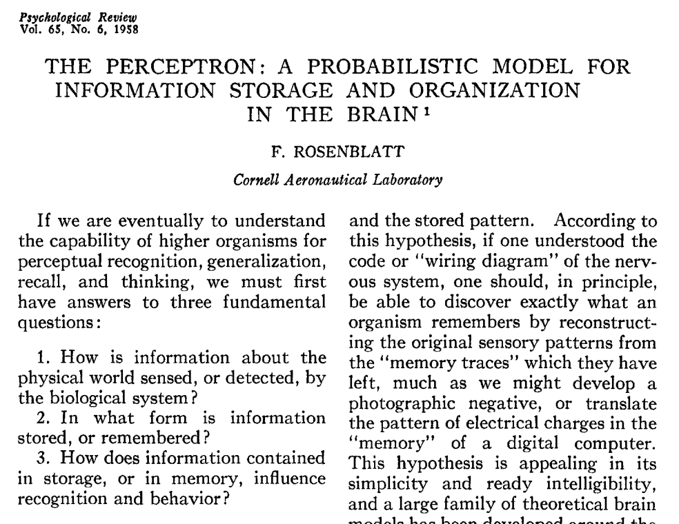
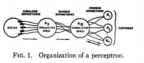
The perceptron algorithm : 1958, Frank Rosenblatt
1958
Perceptron
The perceptron algorithm : 1958, Frank Rosenblatt
.
.
.
output
weights
bias
linear regression:
1958
Perceptron
Perceptrons are linear classifiers: makes its predictions based on a linear predictor function
combining a set of weights (=parameters) with the feature vector.
The perceptron algorithm : 1958, Frank Rosenblatt
x
y
1958
Perceptrons are linear classifiers: makes its predictions based on a linear predictor function
combining a set of weights (=parameters) with the feature vector.
The perceptron algorithm : 1958, Frank Rosenblatt
x
y
1958
Perceptrons are linear classifiers: makes its predictions based on a linear predictor function
combining a set of weights (=parameters) with the feature vector.
The perceptron algorithm : 1958, Frank Rosenblatt
x
y
1958
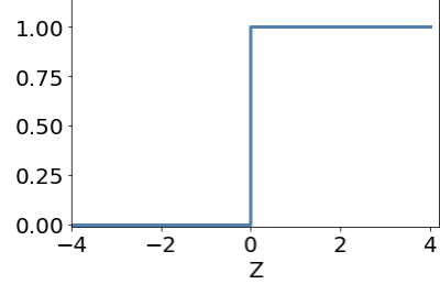
1
0
{
{
.
.
.
output
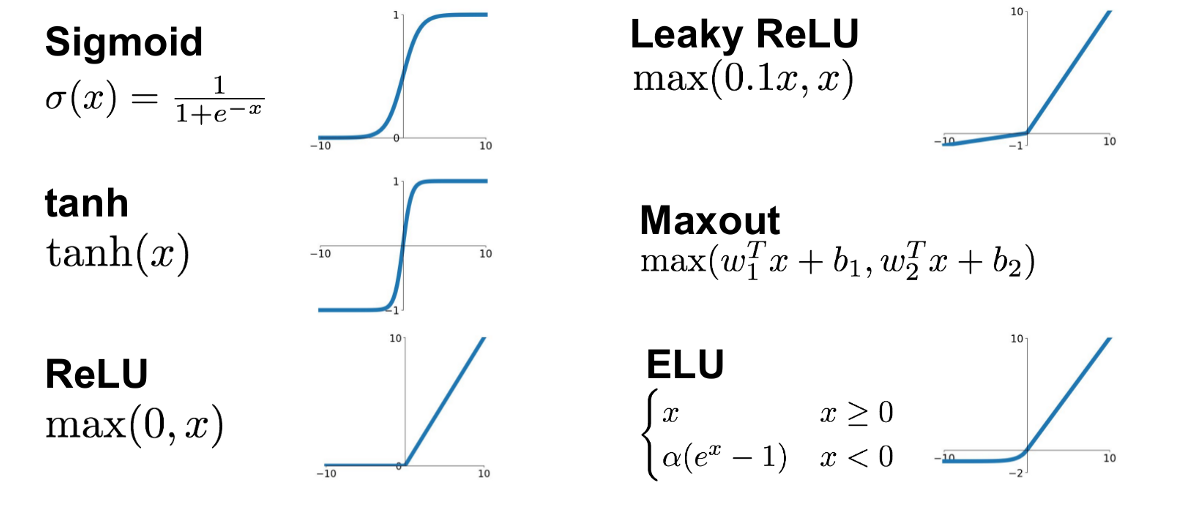
activation function
weights
bias
perceptron
The perceptron algorithm : 1958, Frank Rosenblatt
Perceptrons are linear classifiers: makes its predictions based on a linear predictor function
combining a set of weights (=parameters) with the feature vector.
The perceptron algorithm : 1958, Frank Rosenblatt
output
activation function
weights
bias
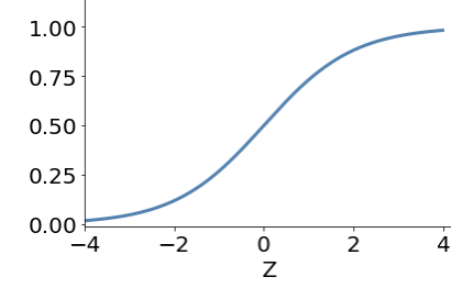
sigmoid
.
.
.
Perceptrons are linear classifiers: makes its predictions based on a linear predictor function
combining a set of weights (=parameters) with the feature vector.
The perceptron algorithm : 1958, Frank Rosenblatt
output
activation function
weights
bias
.
.
.
Perceptron
The perceptron algorithm : 1958, Frank Rosenblatt
Perceptron
The Navy revealed the embryo of an electronic computer today that it expects will be able to walk, talk, see, write, reproduce itself and be conscious of its existence.
The embryo - the Weather Buerau's $2,000,000 "704" computer - learned to differentiate between left and right after 50 attempts in the Navy demonstration
July 8, 1958
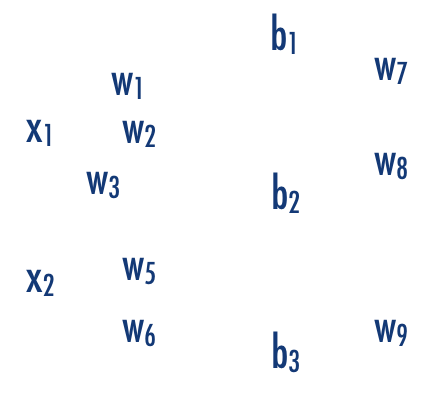
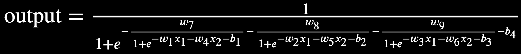
x1
x2
b1
b2
b3
b
w11
w12
w13
w21
w22
w23
w: weight
sets the sensitivity of a neuron
b: bias:
up-down weights a neuron
output
how many parameters?
input layer
hidden layer
output layer
hidden layer
2
output
layer of perceptrons
output
input layer
hidden layer
output layer
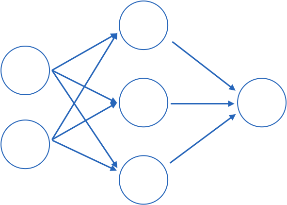
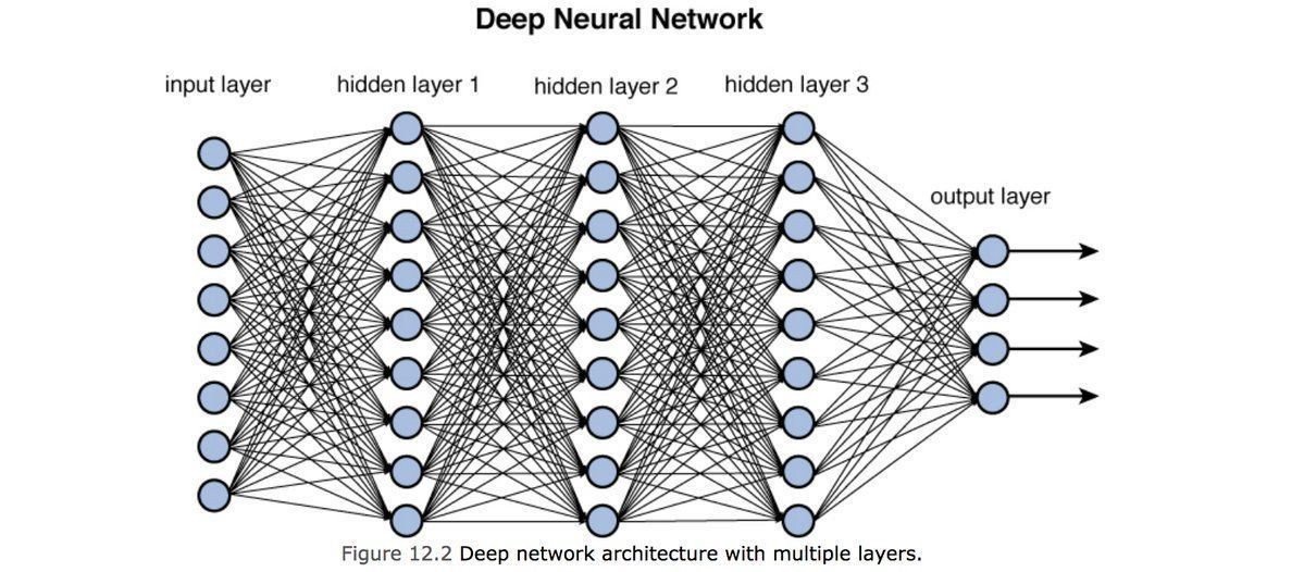
1970: multilayer perceptron architecture
Fully connected: all nodes go to all nodes of the next layer.
output
layer of perceptrons
output
layer of perceptrons
layer of perceptrons
output
layer of perceptrons
output
Fully connected: all nodes go to all nodes of the next layer.
layer of perceptrons
output
Fully connected: all nodes go to all nodes of the next layer.
layer of perceptrons
w: weight
sets the sensitivity of a neuron
b: bias:
up-down weights a neuron
learned parameters
output
Fully connected: all nodes go to all nodes of the next layer.
layer of perceptrons
w: weight
sets the sensitivity of a neuron
b: bias:
up-down weights a neuron
f: activation function:
turns neurons on-off
input layer
hidden layer
output layer
P(0)
P(1)
input layer
hidden layer
output layer
P(C)
P(B)
P(A)
P(D)
input layer
hidden layer
output layer
continuous value
variable
parameters of DNN
3
output
how many parameters?
input layer
hidden layer
output layer
hidden layer
output
how many parameters?
input layer
hidden layer
output layer
hidden layer
3 x 4 (w) + 4 (b) = 16
output
how many parameters?
input layer
hidden layer
output layer
hidden layer
3 x 4 (w) + 4 (b) = 16
4 x 3 (w) + 3 (b) = 15
output
how many parameters?
input layer
hidden layer
output layer
hidden layer
3 x 4 (w) + 4 (b) = 16
4 x 3 (w) + 3 (b) = 15
3 x 1 (w) + 1 (b) = 4
35
hyperparameters of DNN
4
There are other things that change from model to model, but that are not decided based on the data, simply things we decide "a prior"
hyperparameters
output
input layer
hidden layer
output layer
hidden layer
how many hyperparameters?
GREEN: architecture hyperparameters
RED: training hyperparameters
output
input layer
hidden layer
output layer
hidden layer
how many hyperparameters?
GREEN: architecture hyperparameters
RED: training hyperparameters
William of Ockham (logician and Franciscan friar) 1300ca
but probably to be attributed to John Duns Scotus (1265–1308)
“Complexity needs not to be postulated without a need for it”
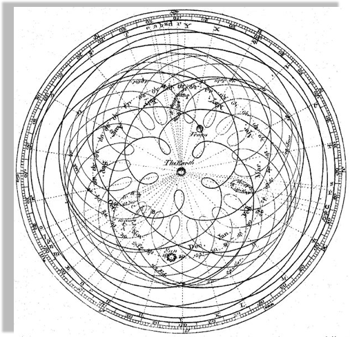
Peter Apian, Cosmographia, Antwerp, 1524 from Edward Grant,
"Celestial Orbs in the Latin Middle Ages", Isis, Vol. 78, No. 2. (Jun., 1987).
Geocentric models are intuitive:
from our perspective we see the Sun moving, while we stay still
the earth is round,
and it orbits around the sun
As observations improve
this model can no longer fit the data!
not easily anyways...
the earth is round,
and it orbits around the sun
Encyclopaedia Brittanica 1st Edition
Dr Long's copy of Cassini, 1777
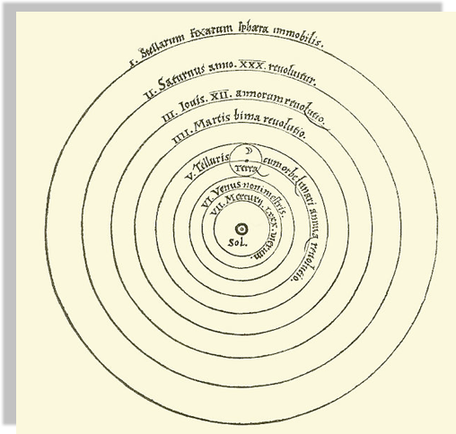
A new model that is much simpler fit the data just as well
(perhaps though only until better data comes...)
the earth is round,
and it orbits around the sun
Heliocentric model from Nicolaus Copernicus' De revolutionibus orbium coelestium.
William of Ockham (logician and Franciscan friar) 1300ca
but probably to be attributed to John Duns Scotus (1265–1308)
“Complexity needs not to be postulated without a need for it”
“Between 2 theories that perform similarly choose the simpler one”
Between 2 theories that perform similarly choose the simpler one
In the context of model selection simpler means "with fewer parameters"
Key Concept
DNN need a lot of data to train
To optimize a lot of parameters we need..... lots of data!
DNN are justified if
- there are a lot of variables
- the relationships between input variables and output are non-linear
4.1
how to make informed choices in the architectural design (TL;DR:... I will offer some guidance, but really you've got to try a bunch of things...)
NN are a vast topics and we only have 2 weeks!
Some FREE references!
michael nielsen
better pedagogical approach, more basic, more clear
ian goodfellow
mathematical approach, more advanced, unfinished
michael nielsen
better pedagogical approach, more basic, more clear
Lots of parameters and lots of hyperparameters! What to choose?
cheatsheet
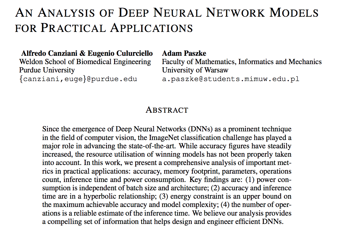
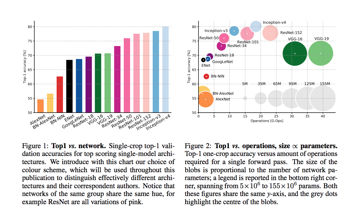
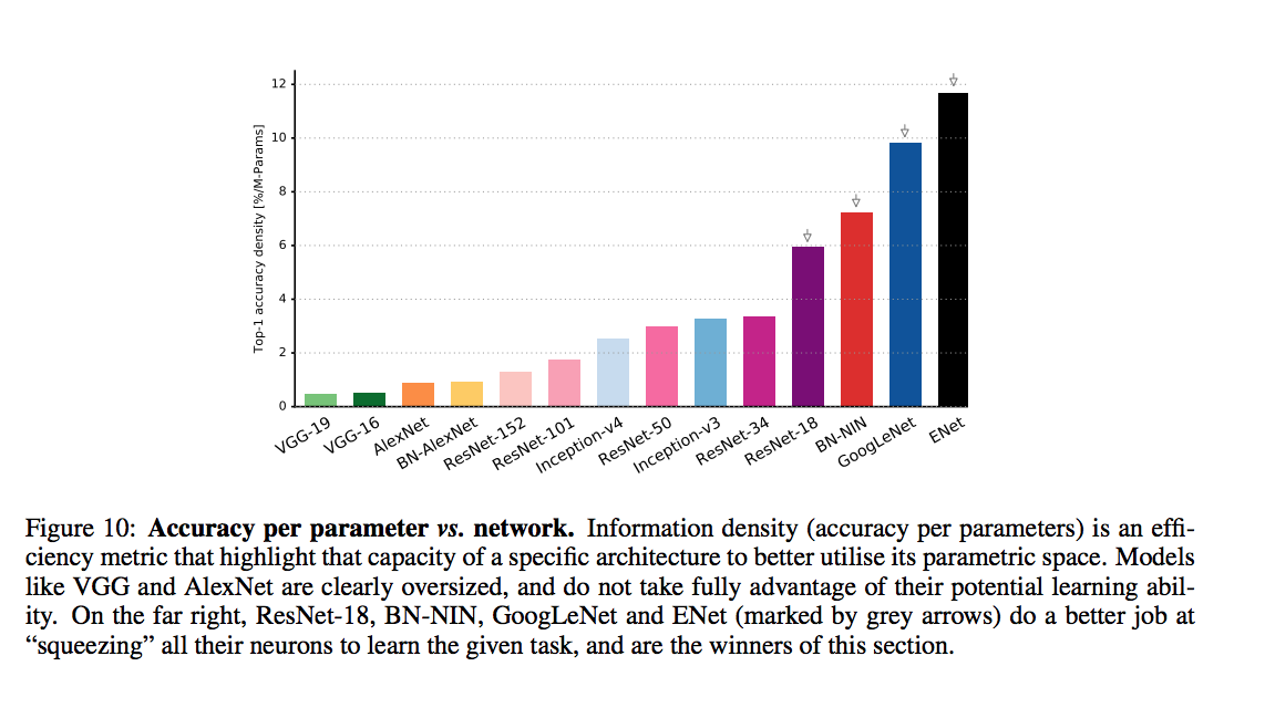
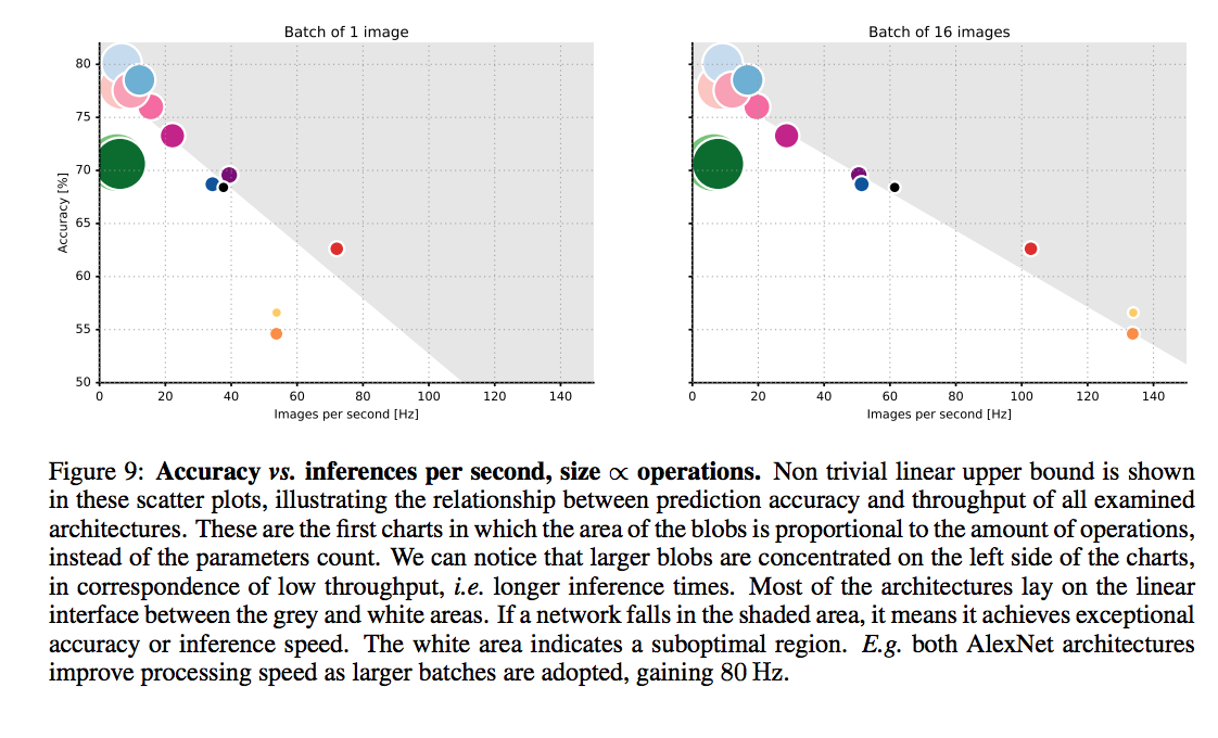
An article that compars various DNNs
An article that compars various DNNs
accuracy comparison
An article that compars various DNNs
accuracy comparison
An article that compars various DNNs
batch size
Lots of parameters and lots of hyperparameters! What to choose?
cheatsheet
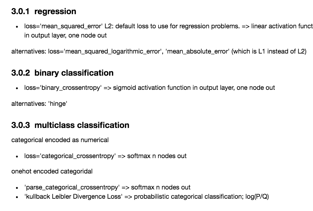
What should I choose for the loss function and how does that relate to the activation functiom and optimization?
Lots of parameters and lots of hyperparameters! What to choose?
Lots of parameters and lots of hyperparameters! What to choose?
cheatsheet
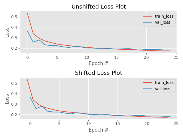
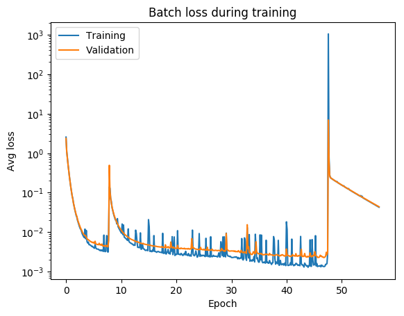
always check your loss function! it should go down smoothly and flatten out at the end of the training.
not flat? you are still learning!
too flat? you are overfitting...
loss (gallery of horrors)
jumps are not unlikely (and not necessarily a problem) if your activations are discontinuous (e.g. relu)
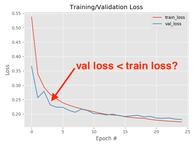
when you use validation you are introducing regularizations (e.g. dropout) so the loss can be smaller than for the training set
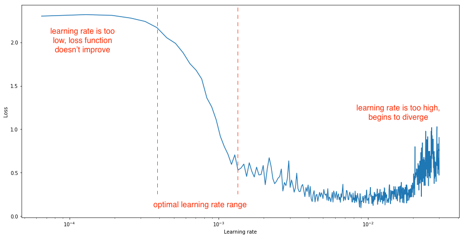
loss and learning rate (not that the appropriate learning rate depends on the chosen optimization scheme!)
Building a DNN
with keras and tensorflow
autoencoder for image recontstruction
What should I choose for the loss function and how does that relate to the activation functiom and optimization?
| loss | good for | activation last layer | size last layer |
|---|---|---|---|
| mean_squared_error | regression | linear | one node |
| mean_absolute_error | regression | linear | one node |
| mean_squared_logarithmit_error | regression | linear | one node |
| binary_crossentropy | binary classification | sigmoid | one node |
| categorical_crossentropy | multiclass classification | sigmoid | N nodes |
| Kullback_Divergence | multiclass classification, probabilistic inerpretation | sigmoid | N nodes |
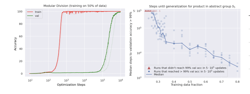
GROKKING: GENERALIZATION BEYOND OVERFITTING ON SMALL ALGORITHMIC DATASETS
For small NNs, it is observed that extending training **well past** the beginning of overfitting can trigger a sudden rapid improve of performance on the test set.
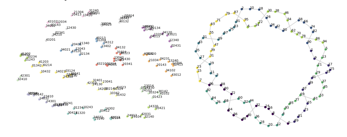
This happens when the latent representation of the data reorganizes itself suddenly in an actually meaningful way. Priori to grokking, the NN is just learning similarities. After grokking, it learns the fundamental relations that govern a phenomenon
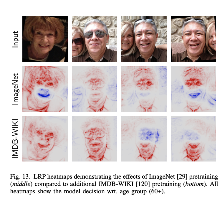
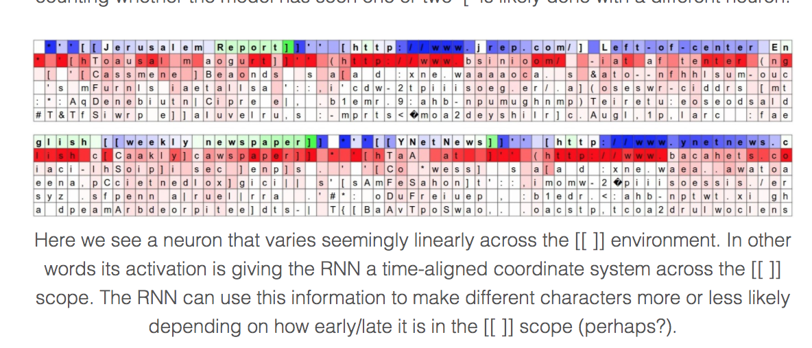
On the interpretability of DNNs
training DNN
5
.
.
.
Any linear model:
y : prediction
ytrue : target
Error: e.g.
intercept
slope
L2
x
Find the best parameters by finding the minimum of the L2 hyperplane
at every step look around and choose the best direction
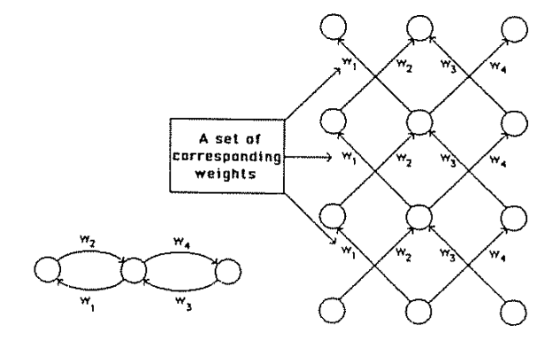
Fully connected: all nodes go to all nodes of the next layer.
1986: Deep Neural Nets
f: activation function:
turns neurons on-off
w: weight
sets the sensitivity of a neuron
b: bias:
up-down weights a neuron
In a CNN these layers would not be fully connected except the last one
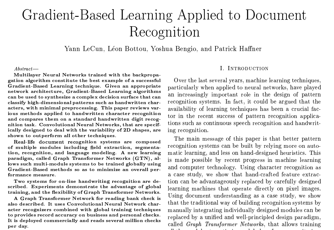
Seminal paper
Y. LeCun 1998
how does linear descent look when you have a whole network structure with hundreds of weights and biases to optimize??
.
.
.
output
Training models with this many parameters requires a lot of care:
. defining the metric
. optimization schemes
. training/validation/testing sets
But just like our simple linear regression case, the fact that small changes in the parameters leads to small changes in the output for the right activation functions.
define a cost function, e.g.
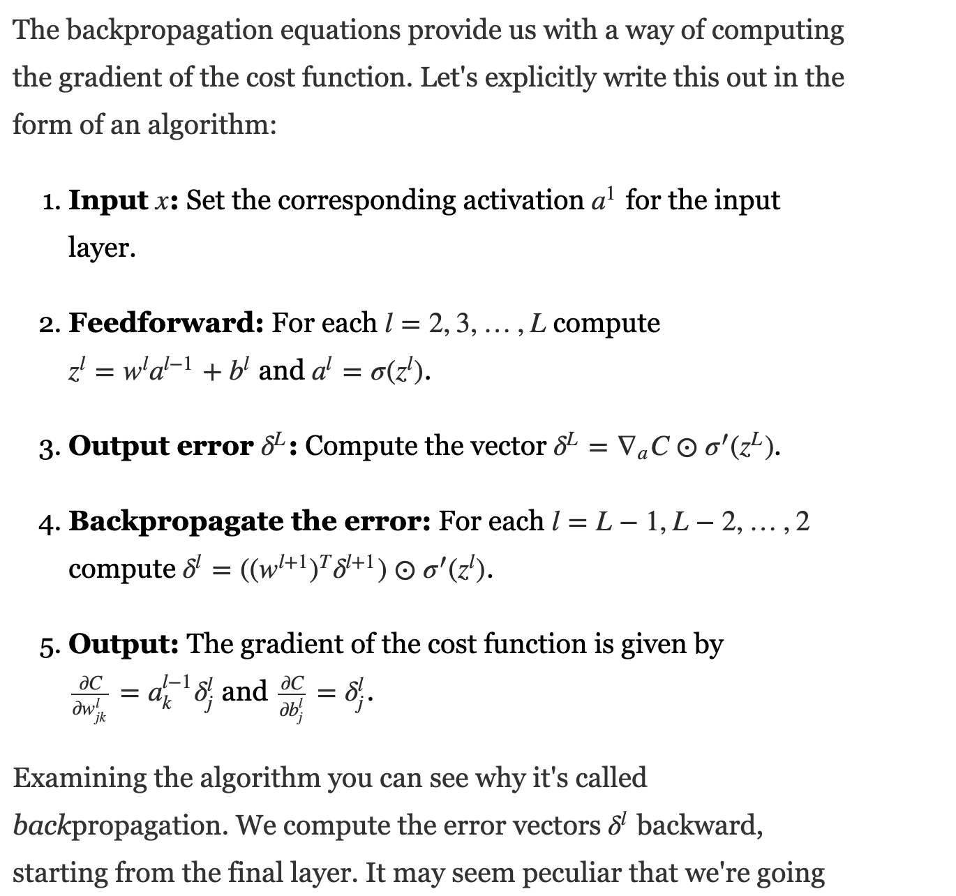
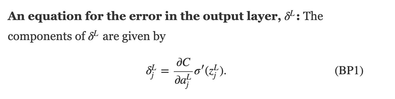
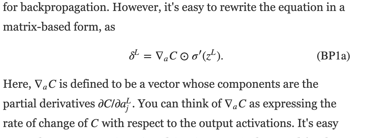
Training a DNN
feed data forward through network and calculate cost metric
for each layer, calculate effect of small changes on next layer
how does linear descent look when you have a whole network structure with hundreds of weights and biases to optimize??
think of applying just gradient to a function of a function of a function... use:
1) partial derivatives, 2) chain rule
define a cost function, e.g.
Training a DNN
Deep Neural Net are not some fancy-pants methods, they are just linear models with a bunch of parameters
Because they have many parameters they are difficult to "interpret" (no easy feature extraction)
that may be ok because they are prediction machines
Because they have many parameters they are difficult to "interpret" (no easy feature extraction)
that may be ok because they are prediction machines
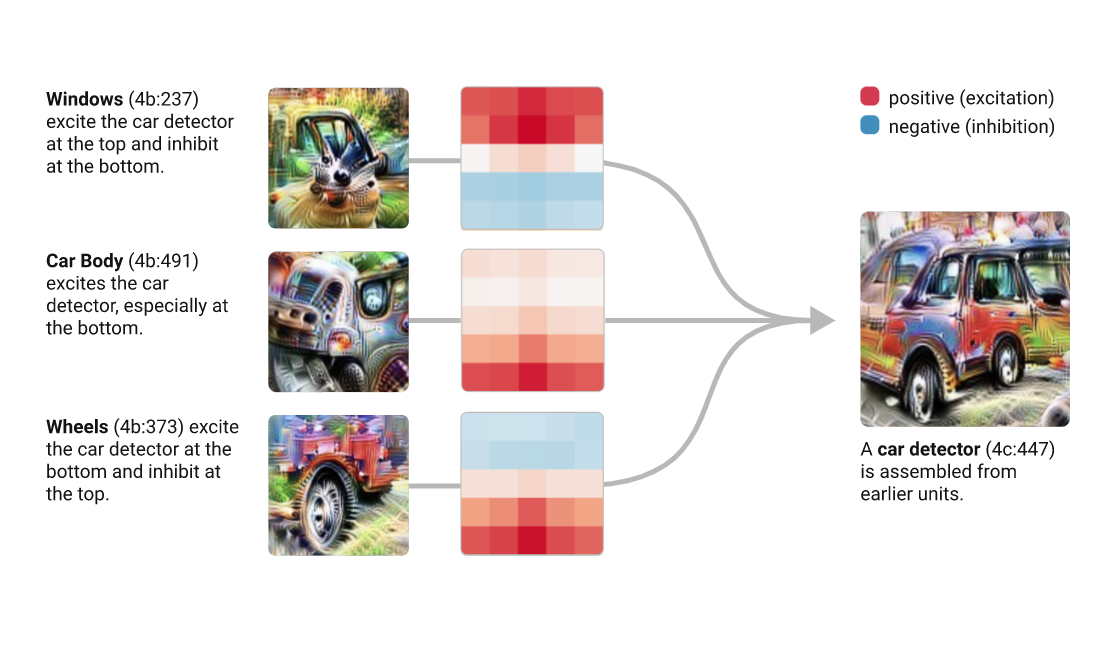
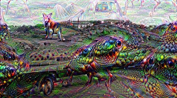
Deep Dream (DD) is a google software, a pre-trained NN (originally created on the Cafe architecture, now imported on many other platforms including tensorflow).
The high level idea relies on training a convolutional NN to recognize common objects, e.g. dogs, cats, cars, in images. As the network learns to recognize those objects is developes its layers to pick out "features" of the NN, like lines at a cetrain orientations, circles, etc.
The DD software runs this NN on an image you give it, and it loops on some layers, thus "manifesting" the things it knows how to recognize in the image.
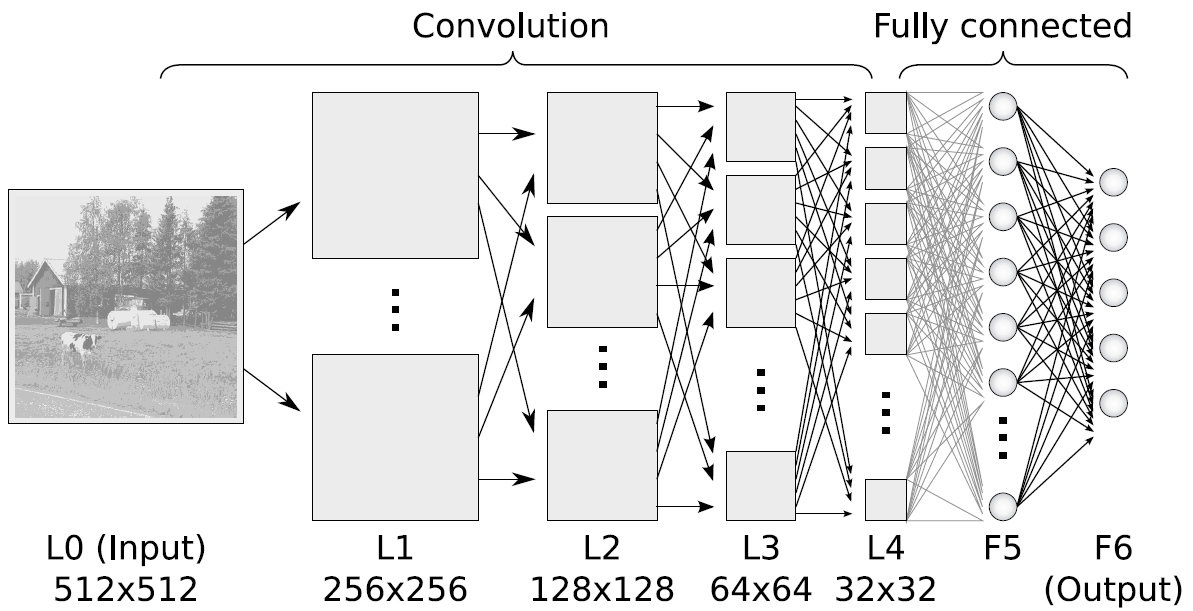
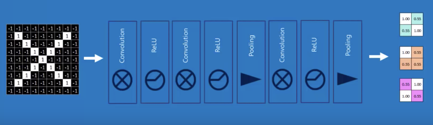
Convolutional Neural Nets
@akumadog
Stack multiple convolution layers
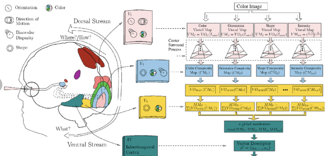
The visual cortex learns hierarchically: first detects simple features, then more complex features and ensembles of features
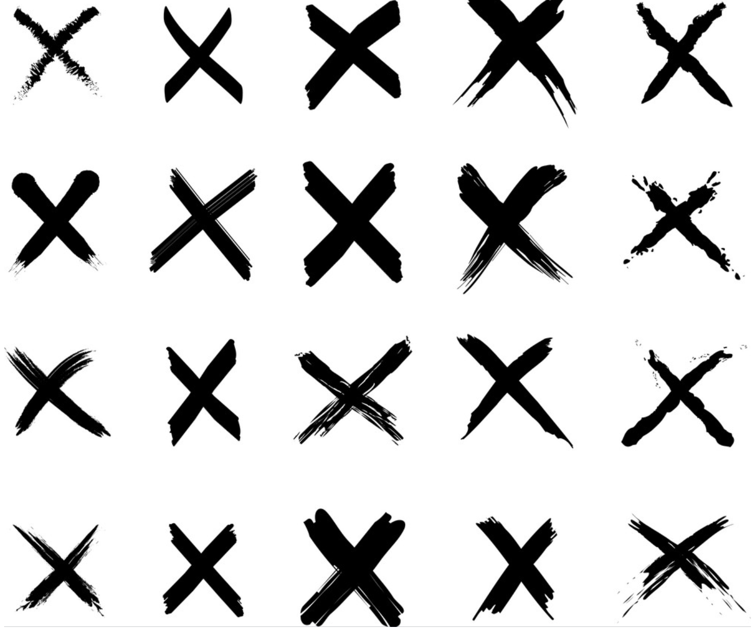
Some shapes are characteristic of the appearance of specific objects:
a dog face is composed of
The visual cortex learns hierarchically: first detects simple features, then more complex features and ensembles of features
a Convolutional NN inspects the images by looking for where the image is maximally similar to the specific form
a dog face is composed of
The visual cortex learns hierarchically: first detects simple features, then more complex features and ensembles of features
a Convolutional NN inspects the images by looking for where the image is maximally similar to the specific form
a dog face is composed of
The visual cortex learns hierarchically: first detects simple features, then more complex features and ensembles of features
a Convolutional NN inspects the images by looking for where the image is maximally similar to the specific form
a dog face is composed of
The visual cortex learns hierarchically: first detects simple features, then more complex features and ensembles of features
a Convolutional NN inspects the images by looking for where the image is maximally similar to the specific form
a dog face is composed of
The visual cortex learns hierarchically: first detects simple features, then more complex features and ensembles of features
a Convolutional NN inspects the images by looking for where the image is maximally similar to the specific form
a dog face is composed of
The visual cortex learns hierarchically: first detects simple features, then more complex features and ensembles of features
a Convolutional NN inspects the images by looking for where the image is maximally similar to the specific form
a dog face is composed of
The visual cortex learns hierarchically: first detects simple features, then more complex features and ensembles of features
Every piece of the image will have a value of similarity with a specified form
a dog face is composed of
The visual cortex learns hierarchically: first detects simple features, then more complex features and ensembles of features
The parameters being learned by the CNN are the template shapes which we call
"convolution kernels"
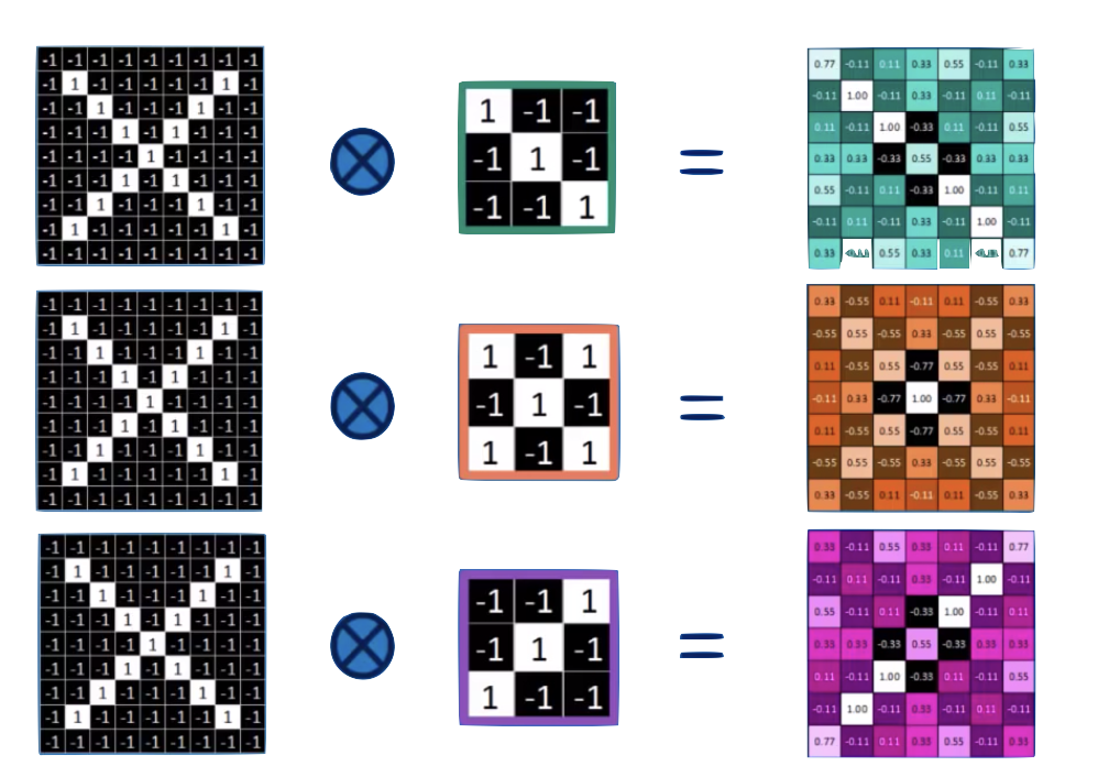
Convolution
Convolution
convolution is a mathematical operator on two functions
f and g
that produces a third function
f x g
expressing how the shape of one is modified by the other.
o
Convolution Theorem
fourier transform
two images.
| -1 | -1 | -1 | -1 | -1 |
|---|---|---|---|---|
| -1 | -1 | -1 | ||
| -1 | -1 | -1 | -1 | |
| -1 | -1 | -1 | ||
| -1 | -1 | -1 | -1 | -1 |
1
1
1
1
1
1
1
1
1
| -1 | -1 | -1 | -1 | -1 |
|---|---|---|---|---|
| -1 | -1 | -1 | -1 | -1 |
| -1 | -1 | -1 | -1 | -1 |
| -1 | -1 | -1 | -1 | -1 |
| -1 | -1 | -1 | -1 | -1 |
| 1 | -1 | -1 |
| -1 | 1 | -1 |
| -1 | -1 | 1 |
1
1
1
1
1
| -1 | -1 | -1 | -1 | -1 |
|---|---|---|---|---|
| -1 | -1 | -1 | ||
| -1 | -1 | -1 | -1 | |
| -1 | -1 | -1 | ||
| -1 | -1 | -1 | -1 | -1 |
| -1 | -1 | 1 |
| -1 | 1 | -1 |
| 1 | -1 | -1 |
feature maps
1
1
1
1
1
convolution
| -1 | -1 | -1 | -1 | -1 |
|---|---|---|---|---|
| -1 | -1 | -1 | ||
| -1 | -1 | -1 | -1 | |
| -1 | -1 | -1 | ||
| -1 | -1 | -1 | -1 | -1 |
| 1 | -1 | -1 |
| -1 | 1 | -1 |
| -1 | -1 | 1 |
1
1
1
1
1
| -1 | -1 | -1 | -1 | -1 |
|---|---|---|---|---|
| -1 | -1 | -1 | ||
| -1 | -1 | -1 | -1 | |
| -1 | -1 | -1 | ||
| -1 | -1 | -1 | -1 | -1 |
| 1 | -1 | -1 |
| -1 | 1 | -1 |
| -1 | -1 | 1 |
| 1 | -1 | -1 |
| -1 | 1 | -1 |
| -1 | -1 | 1 |
| 7 | ||
|---|---|---|
=
1
1
1
1
1
| -1 | -1 | -1 | -1 | -1 |
|---|---|---|---|---|
| -1 | -1 | -1 | ||
| -1 | -1 | -1 | -1 | |
| -1 | -1 | -1 | ||
| -1 | -1 | -1 | -1 | -1 |
| 1 | -1 | -1 |
| -1 | 1 | -1 |
| -1 | -1 | 1 |
| 1 | -1 | -1 |
| -1 | 1 | -1 |
| -1 | -1 | 1 |
| 7 | -3 | |
|---|---|---|
=
1
1
1
1
1
| -1 | -1 | -1 | -1 | -1 |
|---|---|---|---|---|
| -1 | -1 | -1 | ||
| -1 | -1 | -1 | -1 | |
| -1 | -1 | -1 | ||
| -1 | -1 | -1 | -1 | -1 |
| 1 | -1 | -1 |
| -1 | 1 | -1 |
| -1 | -1 | 1 |
| 1 | -1 | -1 |
| -1 | 1 | -1 |
| -1 | -1 | 1 |
| 7 | -3 | 3 |
|---|---|---|
=
1
1
1
1
1
| -1 | -1 | -1 | -1 | -1 |
|---|---|---|---|---|
| -1 | -1 | -1 | ||
| -1 | -1 | -1 | -1 | |
| -1 | -1 | -1 | ||
| -1 | -1 | -1 | -1 | -1 |
| 1 | -1 | -1 |
| -1 | 1 | -1 |
| -1 | -1 | 1 |
| 1 | -1 | -1 |
| -1 | 1 | -1 |
| -1 | -1 | 1 |
| 7 | -3 | 3 |
|---|---|---|
| ? | ||
=
1
1
1
1
1
| -1 | -1 | -1 | -1 | -1 |
|---|---|---|---|---|
| -1 | -1 | -1 | ||
| -1 | -1 | -1 | -1 | |
| -1 | -1 | -1 | ||
| -1 | -1 | -1 | -1 | -1 |
| 1 | -1 | -1 |
| -1 | 1 | -1 |
| -1 | -1 | 1 |
| 1 | -1 | -1 |
| -1 | 1 | -1 |
| -1 | -1 | 1 |
| 7 | -3 | 3 |
|---|---|---|
| ? | ? | |
=
1
1
1
1
1
| -1 | -1 | -1 | -1 | -1 |
|---|---|---|---|---|
| -1 | -1 | -1 | ||
| -1 | -1 | -1 | -1 | |
| -1 | -1 | -1 | ||
| -1 | -1 | -1 | -1 | -1 |
| 1 | -1 | -1 |
| -1 | 1 | -1 |
| -1 | -1 | 1 |
| 1 | -1 | -1 |
| -1 | 1 | -1 |
| -1 | -1 | 1 |
| 7 | -3 | 3 |
|---|---|---|
| ? | ? | |
=
1
1
1
1
1
| -1 | -1 | -1 | -1 | -1 |
|---|---|---|---|---|
| -1 | -1 | -1 | ||
| -1 | -1 | -1 | -1 | |
| -1 | -1 | -1 | ||
| -1 | -1 | -1 | -1 | -1 |
| 1 | -1 | -1 |
| -1 | 1 | -1 |
| -1 | -1 | 1 |
| 1 | -1 | -1 |
| -1 | 1 | -1 |
| -1 | -1 | 1 |
| 7 | -3 | 3 |
|---|---|---|
| ? | ? | |
=
1
1
1
1
1
| -1 | -1 | -1 | -1 | -1 |
|---|---|---|---|---|
| -1 | -1 | -1 | ||
| -1 | -1 | -1 | -1 | |
| -1 | -1 | -1 | ||
| -1 | -1 | -1 | -1 | -1 |
| 1 | -1 | -1 |
| -1 | 1 | -1 |
| -1 | -1 | 1 |
| 1 | -1 | -1 |
| -1 | 1 | -1 |
| -1 | -1 | 1 |
| 7 | -3 | 3 |
|---|---|---|
| ? | ? | |
=
1
1
1
1
1
| -1 | -1 | -1 | -1 | -1 |
|---|---|---|---|---|
| -1 | -1 | -1 | ||
| -1 | -1 | -1 | -1 | |
| -1 | -1 | -1 | ||
| -1 | -1 | -1 | -1 | -1 |
| 1 | -1 | -1 |
| -1 | 1 | -1 |
| -1 | -1 | 1 |
| 1 | -1 | -1 |
| -1 | 1 | -1 |
| -1 | -1 | 1 |
| 7 | -3 | 3 |
|---|---|---|
| ? | ? | |
=
1
1
1
1
1
| -1 | -1 | -1 | -1 | -1 |
|---|---|---|---|---|
| -1 | -1 | -1 | ||
| -1 | -1 | -1 | -1 | |
| -1 | -1 | -1 | ||
| -1 | -1 | -1 | -1 | -1 |
| 1 | -1 | -1 |
| -1 | 1 | -1 |
| -1 | -1 | 1 |
| 7 | -3 | 3 |
|---|---|---|
| -3 | ||
=
input layer
feature map
convolution layer
1
1
1
1
1
| -1 | -1 | -1 | -1 | -1 |
|---|---|---|---|---|
| -1 | -1 | -1 | ||
| -1 | -1 | -1 | -1 | |
| -1 | -1 | -1 | ||
| -1 | -1 | -1 | -1 | -1 |
| 1 | -1 | -1 |
| -1 | 1 | -1 |
| -1 | -1 | 1 |
| 7 | -3 | 3 |
| -3 | 5 | -3 |
| 3 | -3 | 7 |
=
input layer
feature map
convolution layer
the feature map is "richer": we went from binary to R
1
1
1
1
1
| -1 | -1 | -1 | -1 | -1 |
|---|---|---|---|---|
| -1 | -1 | -1 | ||
| -1 | -1 | -1 | -1 | |
| -1 | -1 | -1 | ||
| -1 | -1 | -1 | -1 | -1 |
| 1 | -1 | -1 |
| -1 | 1 | -1 |
| -1 | -1 | 1 |
=
input layer
feature map
convolution layer
the feature map is "richer": we went from binary to R
and it is reminiscent of the original layer
7
5
7
| 7 | -3 | 3 |
| -3 | 5 | -3 |
| 3 | -3 | 7 |
=
7
7
Convolve with different feature: each neuron is 1 feature
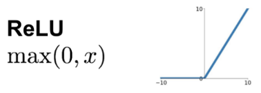
ReLu
| 7 | -3 | 3 |
| -5 | 5 | -3 |
| -6 | -1 | 7 |
7
5
7
ReLu: normalization that replaces negative values with 0's
| 7 | 0 | 3 |
| 0 | 5 | 0 |
| 3 | 0 | 7 |
7
5
7
Max-Pool
MaxPooling: reduce image size, generalizes result
| 7 | 0 | 3 |
| 0 | 5 | 0 |
| 3 | 0 | 7 |
7
5
7
MaxPooling: reduce image size, generalizes result
| 7 | 0 | 3 |
| 0 | 5 | 0 |
| 3 | 0 | 7 |
7
5
7
2x2 Max Poll
| 7 | 5 |
MaxPooling: reduce image size, generalizes result
| 7 | 0 | 3 |
| 0 | 5 | 0 |
| 3 | 0 | 7 |
7
5
7
2x2 Max Poll
| 7 | 5 |
| 5 |
MaxPooling: reduce image size, generalizes result
| 7 | 0 | 3 |
| 0 | 5 | 0 |
| 3 | 0 | 7 |
7
5
7
2x2 Max Poll
| 7 | 5 |
| 5 | 7 |
MaxPooling: reduce image size & generalizes result
By reducing the size and picking the maximum of a sub-region we make the network less sensitive to specific details
x
O
last hidden layer
output layer
Neural Network and Deep Learning
an excellent and free book on NN and DL
http://neuralnetworksanddeeplearning.com/index.html
History of NN
https://cs.stanford.edu/people/eroberts/courses/soco/projects/neural-networks/History/history2.html
By federica bianco


