


federica bianco PRO
astro | data science | data for good
dr.federica bianco | fbb.space | fedhere | fedhere
II: probability and statistics
Recap
Improving Decision Making through Data
Improving Decision Making through Data
It is estimated that the amount of data collected by humans from the beginning of history through 2003 is 5 exabytes.
Improving Decision Making through Data
It is estimated that the amount of data collected by humans from the beginning of history through 2003 is 5 exabytes.
Since 2013 humans generate and store ~5 exabytes of data every day
Improving Decision Making through Data
It is estimated that the amount of data collected by humans from the beginning of history through 2003 is 5 exabytes.
Since 2013 humans generate and store ~5 exabytes of data every day
how do i maximize information from few datapoints
how do i extract the critical informatoin and throw away unnecessary content from big data
Improving Decision Making through Data
Pattern Extraction
Data Collection
Interpretation
Pattern Extraction
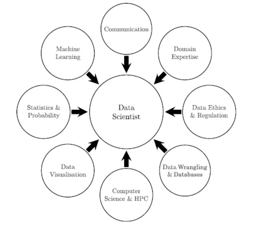
Data Science - Kelleher & Tierney
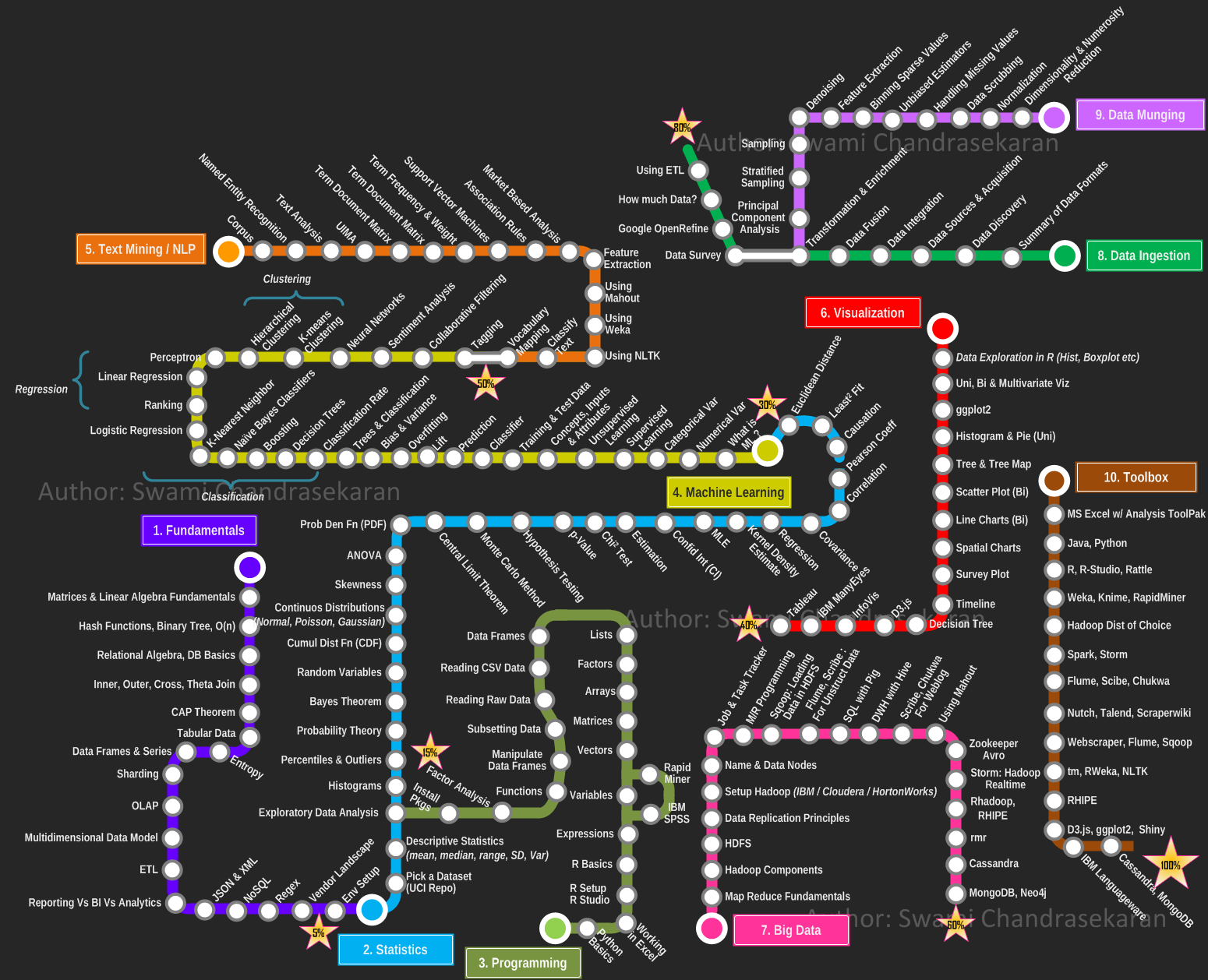
Machine Learning
Stats and Probability
Data Visualization
Computer Science / HPC
Data Wrangling
& Databases
Data Ethics
& Regulation
Domain Expertise
Communication
tech skills
comm skills
additional
skills
Improving Decision Making through Data
Pattern Extraction
Data Collection
Interpretation
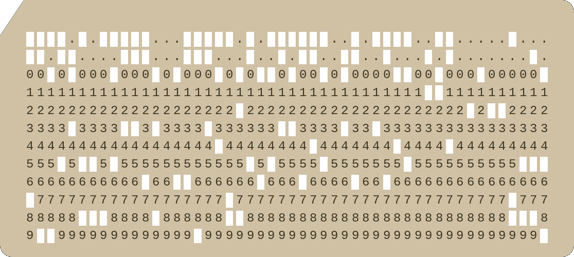
1750
punch cards
BC
1975 E.Cobb
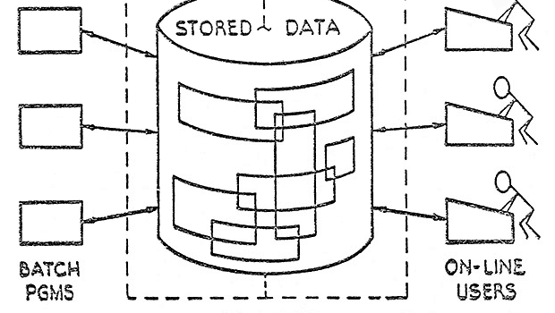
Relational DataBases (SQL)
information could be accessed without knowing how the information was structured or where it resided in the database.
Improving Decision Making through Data
Pattern Extraction
Data Collection
Interpretation
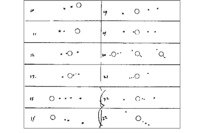
a natural human tendency!
likely an evolutionary advantage
Improving Decision Making through Data
Data Collection
Interpretation
Pattern Extraction
Improving Decision Making through Data
Data Collection
Interpretation
Pattern Extraction
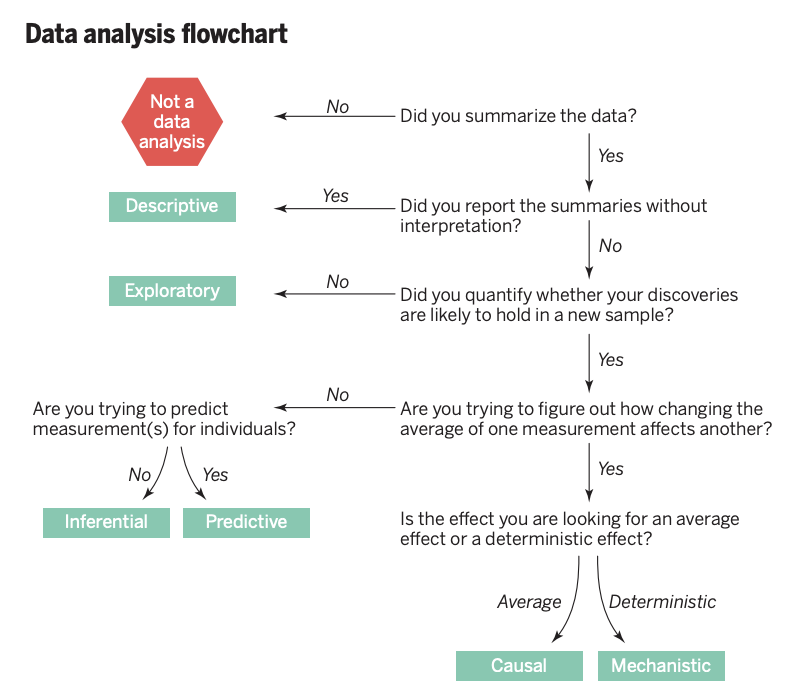
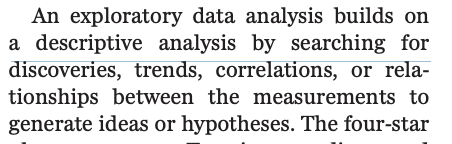
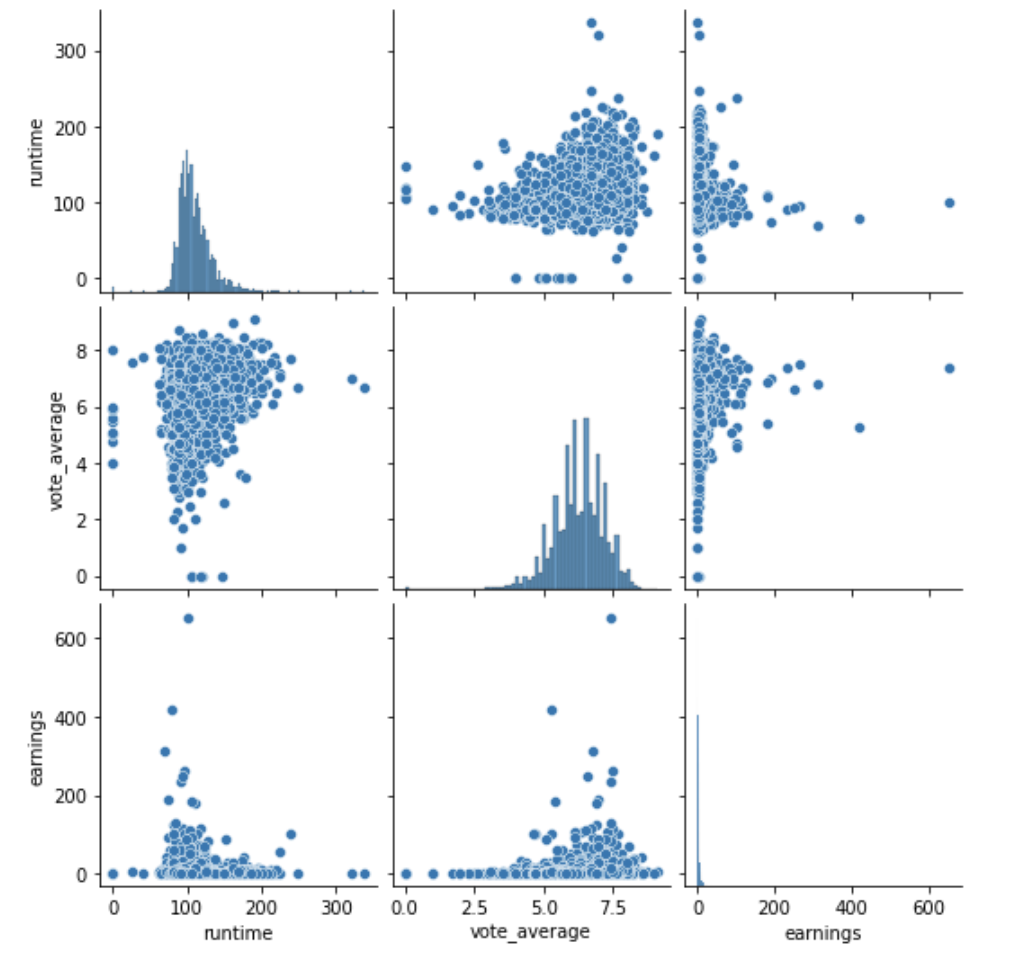
the steps of data-analysis and inference: descriptive and exploratory analysis
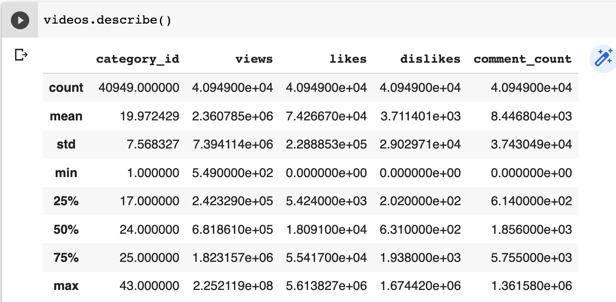
import pandas as pd
df = pd.read_csv(file_name)
df.describe()
- how is data organized
- is data complete?
- what are the statistical properties of the data
we will look at the statistical properties: mean, standard deviation, median, quantiles...
- searching for anomalies, trends
- searching for relationships between the measurements (correlation)
Inferential: will patterns hold?
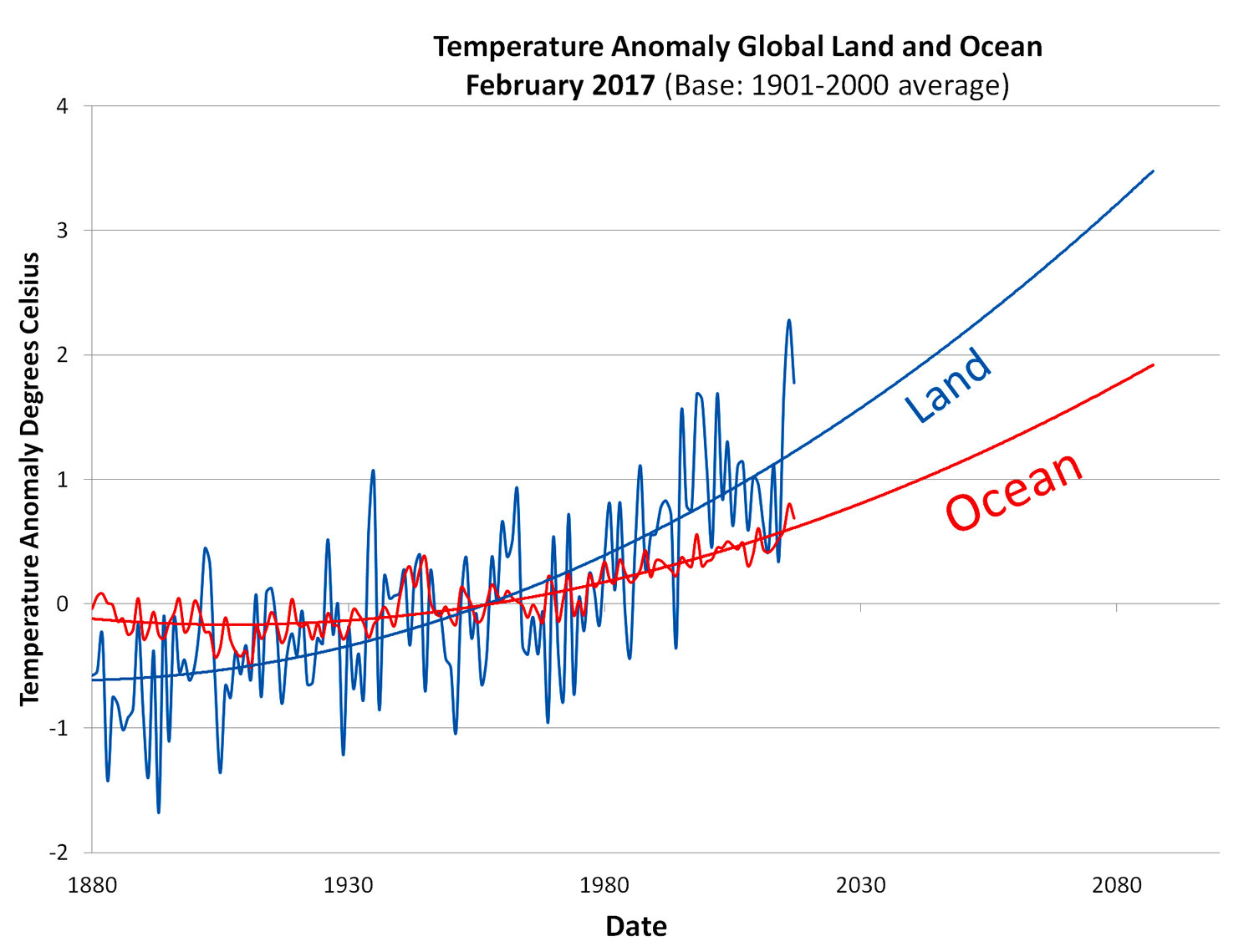
Predictive: what will be the temperature in 2030?
Causal: is the cause of the heating of the earth? CO2? Solar Cycles?
Data Science Practices
3 General principles of "good" science
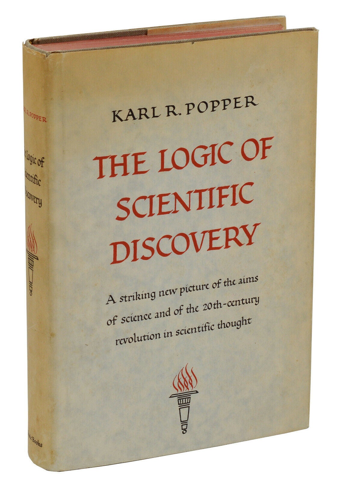
Falisifiability
Parsimony
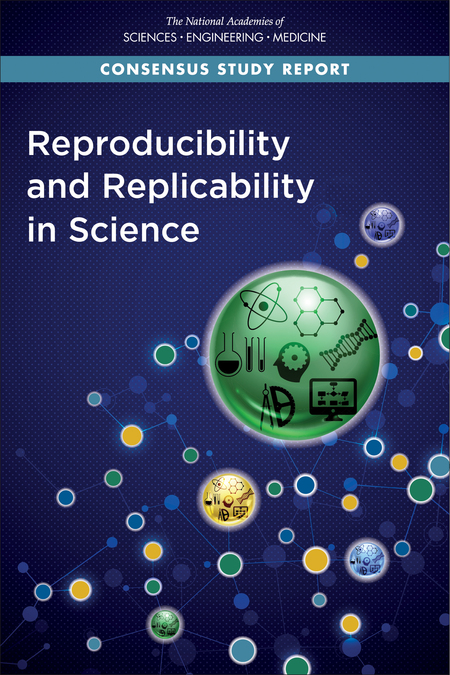
Reproducibility
Reproducible research means:
all numbers in a data analysis can be recalculated exactly (down to stochastic variables!) using the code and raw data provided by the analyst.
Claerbout, J. 1990,
Active Documents and Reproducible Results, Stanford Exploration Project Report, 67, 139
allows reproducibility through code distribution
Reproducible research means:
the ability of a researcher to duplicate the results of a prior study using the same materials as were used by the original investigator. That is, a second researcher might use the same raw data to build the same analysis files and implement the same statistical analysis in an attempt to yield the same results.
assures a result is grounded in evidence
1
#openscience
#opendata
Reproducible research means:
the ability of a researcher to duplicate the results of a prior study using the same materials as were used by the original investigator. That is, a second researcher might use the same raw data to build the same analysis files and implement the same statistical analysis in an attempt to yield the same results.
facilitates scientific progress by avoiding the need to duplicate unoriginal research
2
Reproducible research means:
the ability of a researcher to duplicate the results of a prior study using the same materials as were used by the original investigator. That is, a second researcher might use the same raw data to build the same analysis files and implement the same statistical analysis in an attempt to yield the same results.
facilitate collaboration and teamwork
3
Reproducible research means:
the ability of a researcher to duplicate the results of a prior study using the same materials as were used by the original investigator. That is, a second researcher might use the same raw data to build the same analysis files and implement the same statistical analysis in an attempt to yield the same results.
Reproducible research in practice:
using the code and raw data provided by the analyst.
all numbers in a data analysis can be recalculated exactly (down to stochastic variables!)
see slides week 1:
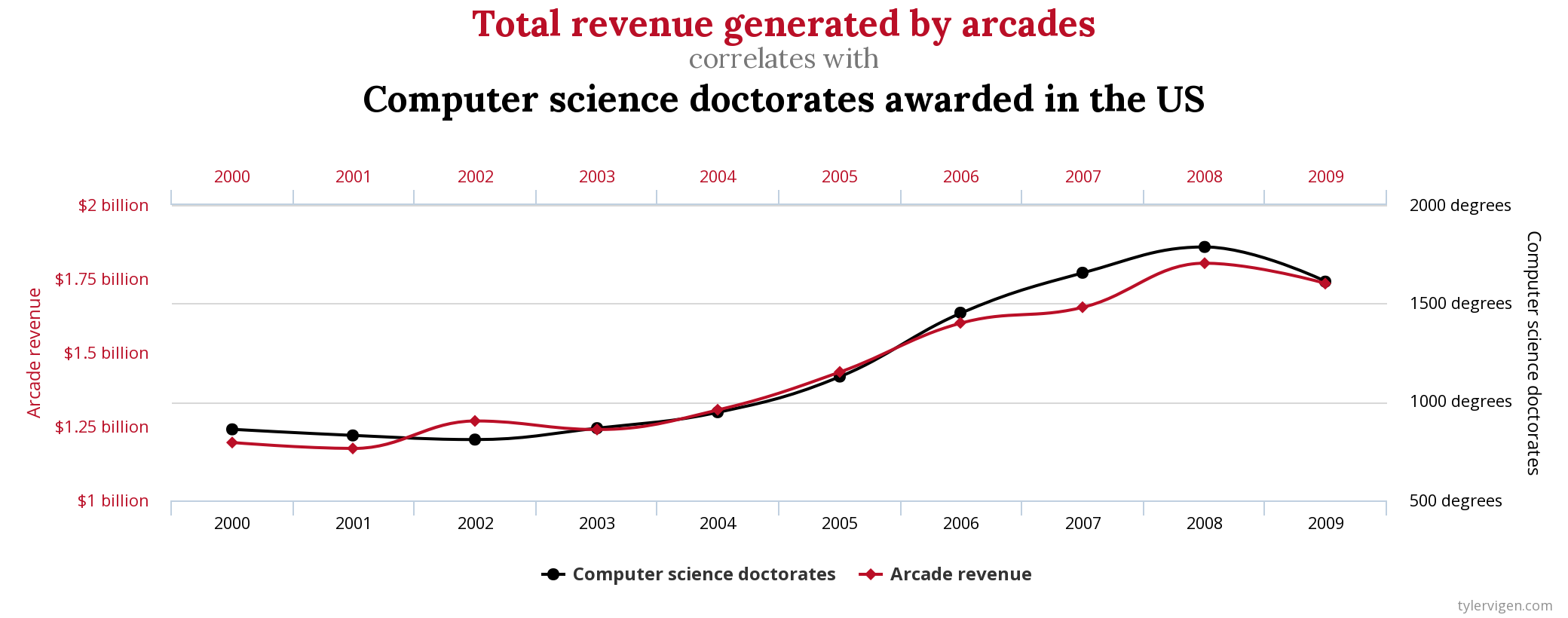
Correlation does not imply causality!!
2 things may be related because they share a cause but not cause each other:
icecream sales with temperature |death by drowning
with temperature
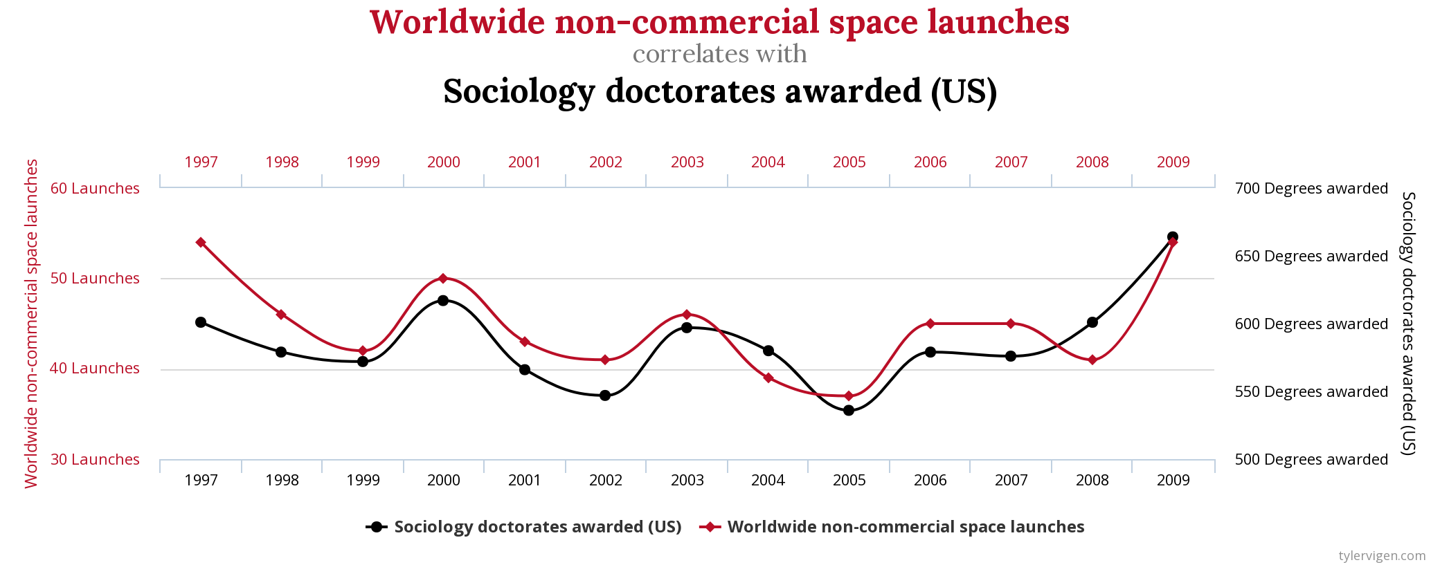
In the era of big data you may encounter truly spurious correlations
divorce rate in Maine | consumption of Margarine
what is Data Science
EXPLORATORY DATA ANALYSIS
Correlation does not imply causality!!
2 things may be related because they share a cause but not cause each other:
icecream sales with temperature |death by drowning
with temperature
In the era of big data you may encounter truly spurious correlations
divorce rate in Maine | consumption of Margarine
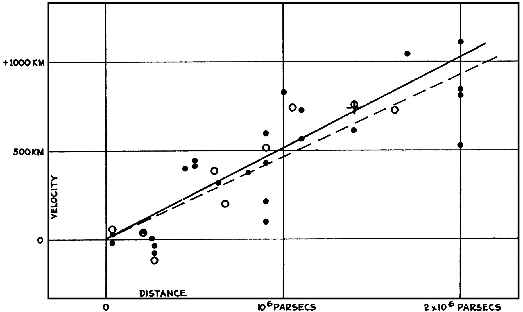
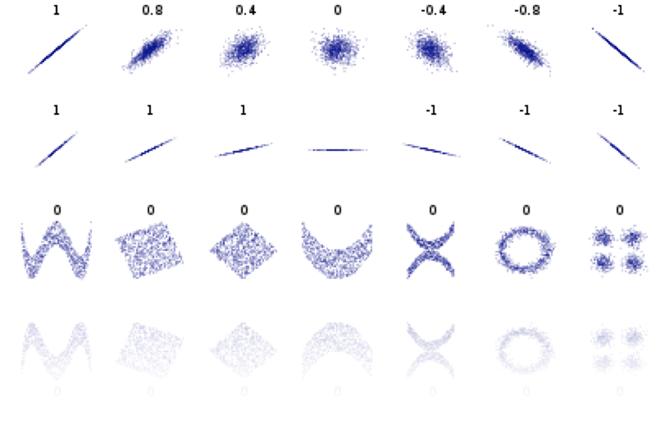
Pearson's correlation
Pearson's correlation measures linear correlation
Pearson's correlation
Pearson's correlation measures linear correlation
correlated
"positively" correlated
Pearson's correlation
Pearson's correlation measures linear correlation
correlated
"positively" correlated
Pearson's correlation
Pearson's correlation measures linear correlation
anticorrelated
"negatively" correlated
Pearson's correlation
Pearson's correlation measures linear correlation
anticorrelated
"negatively" correlated
Pearson's correlation
Pearson's correlation measures linear correlation
not linearly correlated
Pearson's coefficient = 0
does not mean that x and y are independent!
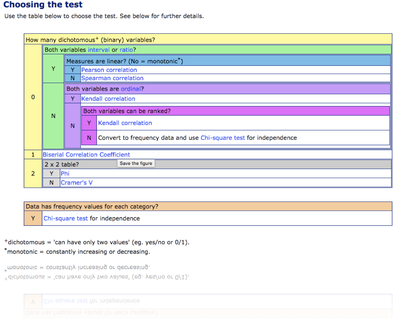
Pearson's correlation
Spearman's test
(Pearson's for ranked values)
Pearson's correlation
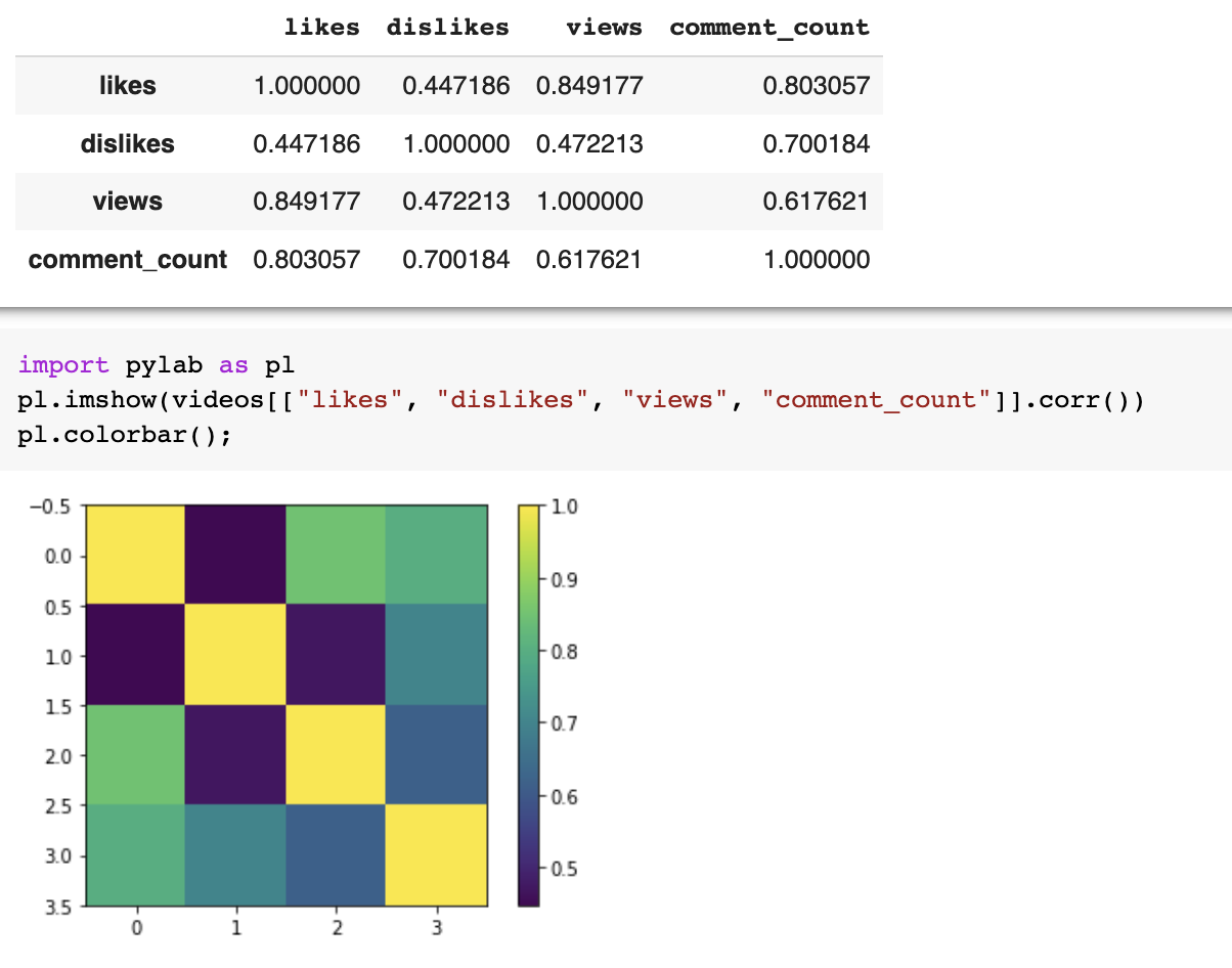
import pandas as pd
df = pd.read_csv(file_name)
df.corr()import pandas as pd
df = pd.read_csv(file_name)
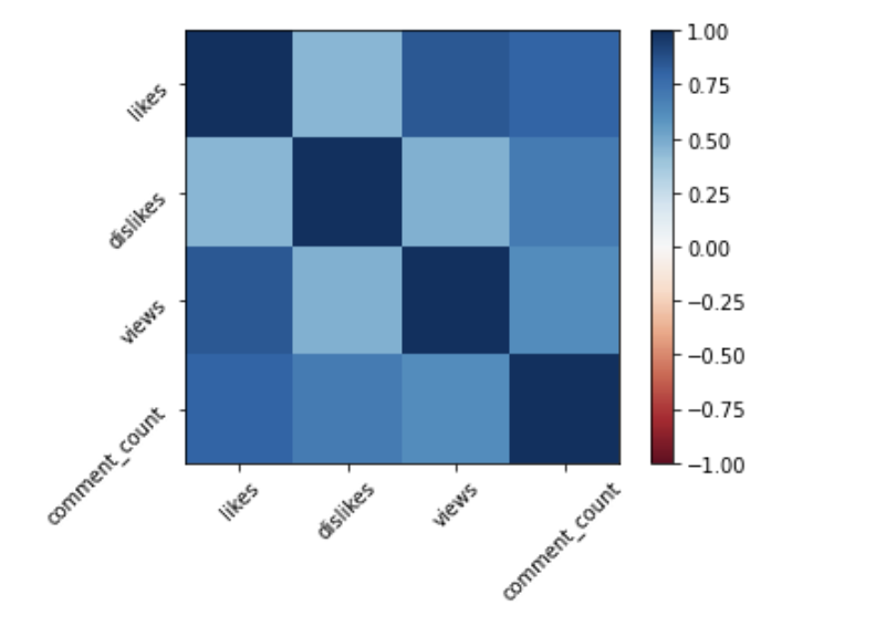
df.corr()pl.imshow(vdf.corr(), clim=(-1,1), cmap='RdBu')
pl.xticks(list(range(len(df.corr()))),
df.columns, rotation=45)
pl.yticks(list(range(len(df.corr()))),
df.columns, rotation=45)
pl.colorbar();<- anticorrelated | correlated ->
probability
Crush Course in Statistics
freee statistics book: http://onlinestatbook.com/
fraction of times something happens
probability of it happening
represents a level of certainty relating to a potential outcome or idea:
if I believe the coin is unfair (tricked) then even if I get a head and a tail I will still believe I am more likely to get heads than tails
<=>
fraction of times something happens
probability of it happening
<=>
P(E) = frequency of E
P(coin = head) = 6/11 = 0.55
fraction of times something happens
probability of it happening
<=>
P(coin = head) = 51/101 = 0.504
P(E) = frequency of E
P(coin = head) = 6/11 = 0.55
Probability Arithmetic
A
B
Rules:
Probability Arithmetic
A
B
Rules:
(everything but A)
Probability Arithmetic
disjoint events:
independent probabilities
A
B
Probability Arithmetic
A
B
related events:
dependent probabilities
Probability Arithmetic
dependent probabilities
A
B
statistics
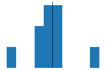
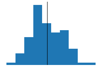
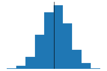
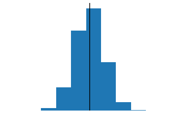
A distribution is a collection of datapoints whose frequency in the sample corresponds to a known formula
parameters (lambda=1)
support
A number k (e.g. 1) has some probability of being drawn
The probability depents on the parameters of the distribution λ
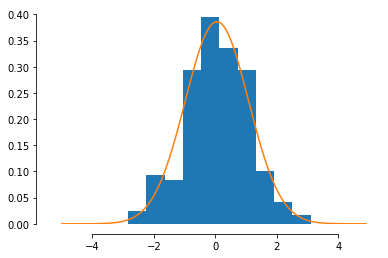
If I draw N numbers and plot a histogram of them the histogram will have a specific shape
parameters (-0.1, 0.9)
support
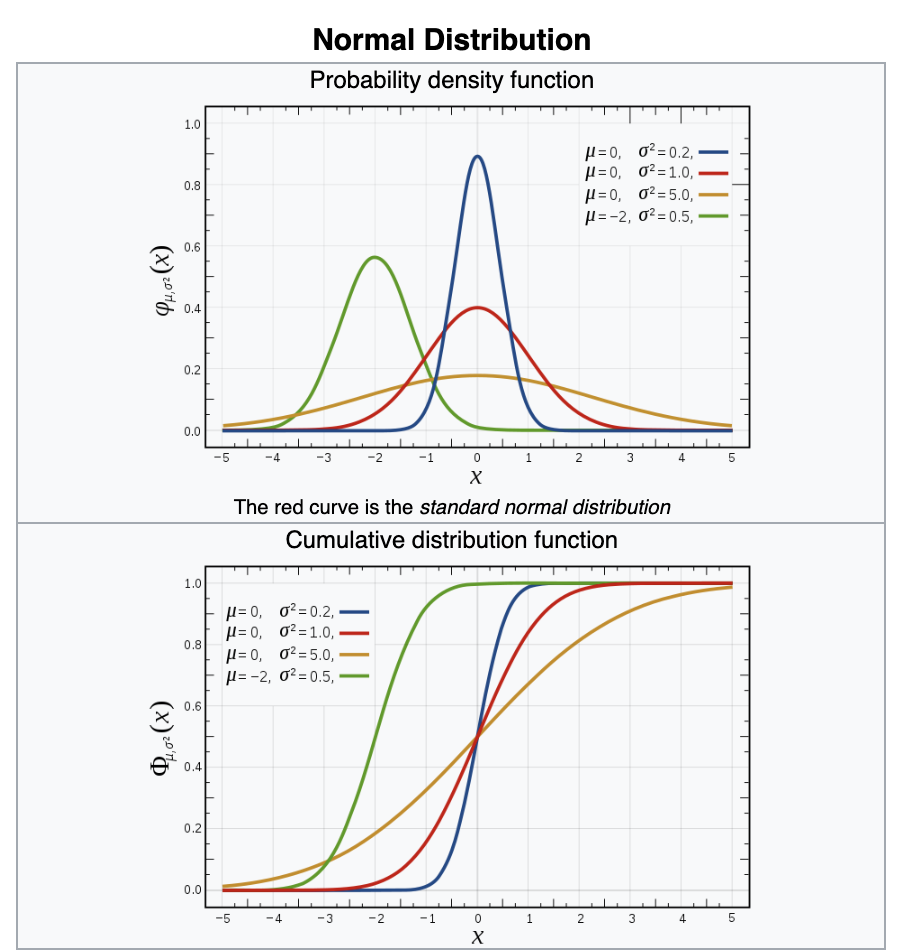
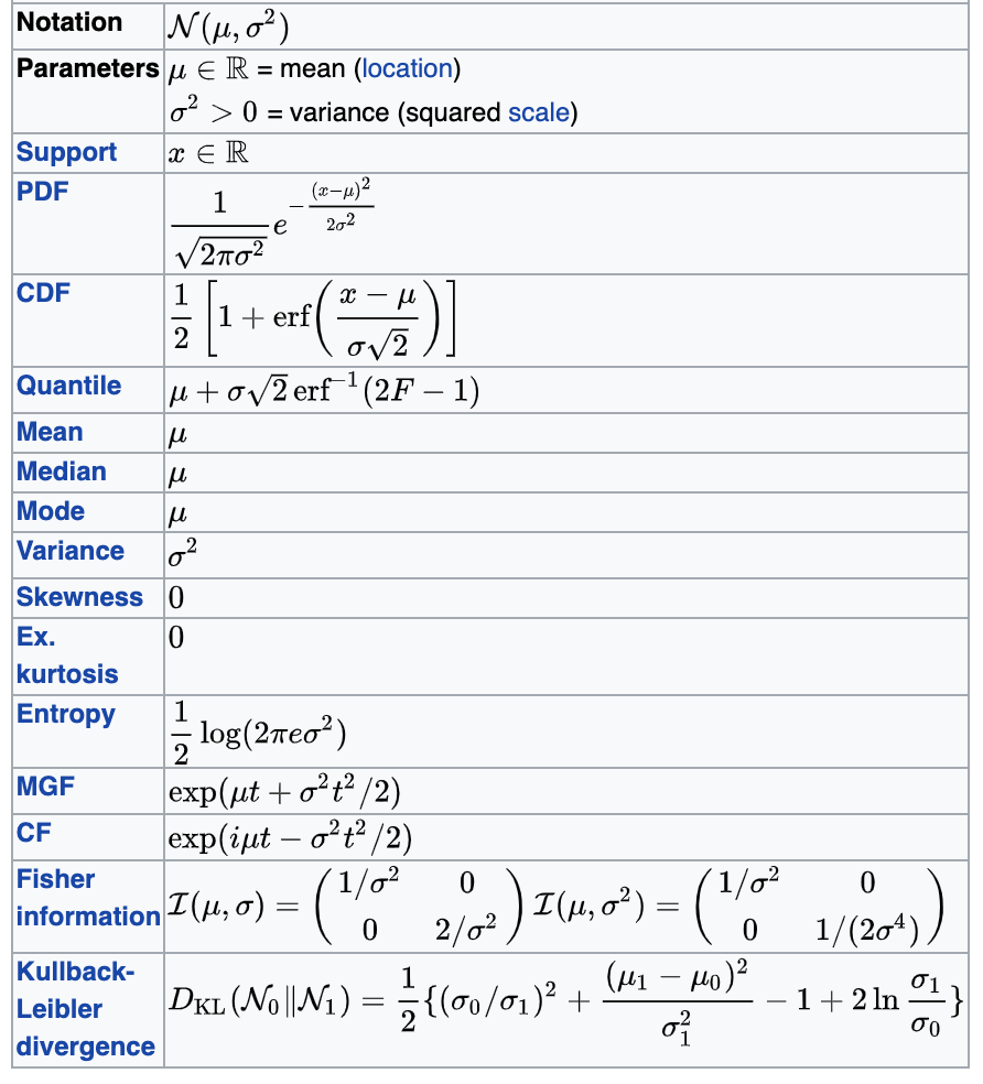
normal or Gaussian
continuous support
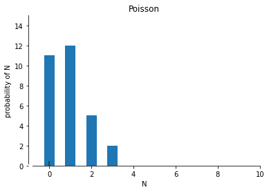
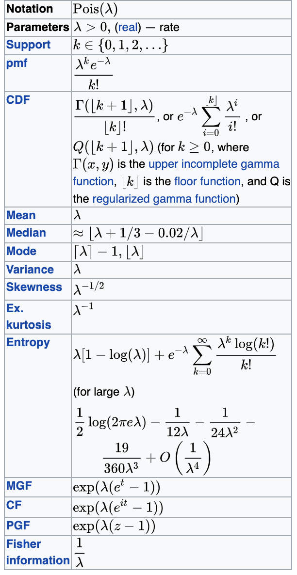
Poisson
discrete support (only ints)
a distribution’s moments summarize its properties:
central tendency: mean (n=1), median, mode
spread: standard deviation/variance (n=2), quartiles range
symmetry: skewness (n=3)
cuspiness: kurtosis (n=4)
a distribution’s moments summarize its properties:
central tendency: mean (n=1), median, mode
spread: standard deviation/variance (n=2), quartiles range
symmetry: skewness (n=3)
cuspiness: kurtosis (n=4)
a distribution’s moments summarize its properties:
central tendency: mean (n=1), median, mode
spread: standard deviation/variance (n=2), quartiles range
symmetry: skewness (n=3)
cuspiness: kurtosis (n=4)
a distribution’s moments summarize its properties:
central tendency: mean (n=1), median, mode
spread: standard deviation/variance (n=2), quartiles range
symmetry: skewness (n=3)
cuspiness: kurtosis (n=4)
Law of Large Numbers
As the size of a _____________ tends to infinity the mean of the sample tends to the mean of the _______________
Laplace (1700s) but also: Poisson, Bessel, Dirichlet, Cauchy, Ellis
Let X1...XN be an N-elements sample from a population whose distribution has
mean μ and standard deviation σ
In the limit of N -> infinity
the sample mean x approaches a Normal (Gaussian) distribution with mean μ and standard deviation σ
regardless of the distribution of X
Central Limit Theorem
HW
extra
credits
Coin toss:
fair coin: p=0.5 n=1
Vegas coin: p=0.5 n=1
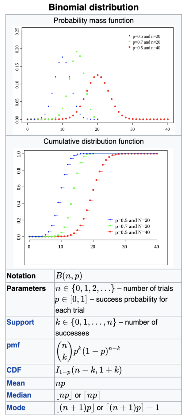
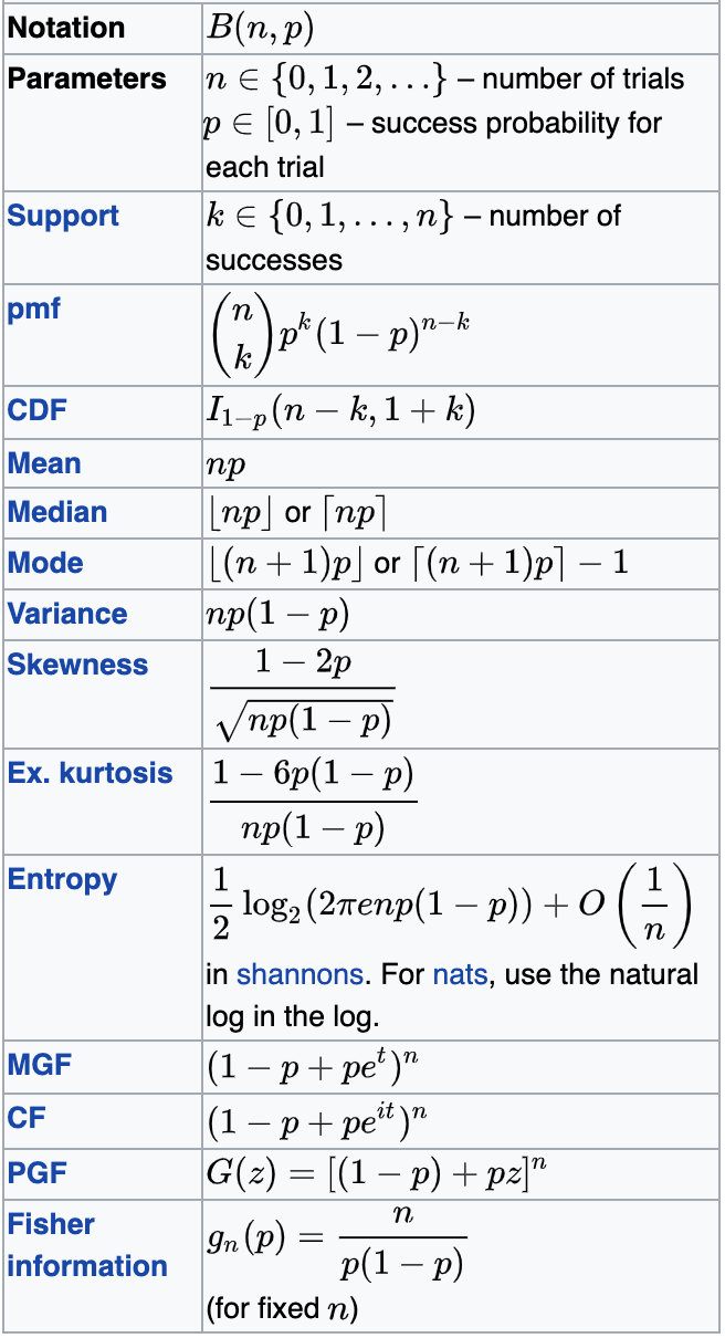
Binomial
I bet heads:
head = success
"given n tosses, each with a probability of 0.5 to get head"
Coin toss:
fair coin: p=0.5 n=1
Vegas coin: p=0.5 n=1
Binomial
Coin toss:
fair coin: p=0.5 n=1
Vegas coin: p=0.5 n=1
Binomial
Coin toss:
fair coin: p=0.5 n=1
Vegas coin: p=0.5 n=1
Binomial
central tendency
np=mean
Coin toss:
fair coin: p=0.5 n=1
Vegas coin: p=0.5 n=1
Binomial
np(1-p)=variance
Binomial
Coin toss:
fair coin: p=0.5 n=1
Vegas coin: p=0.5 n=1
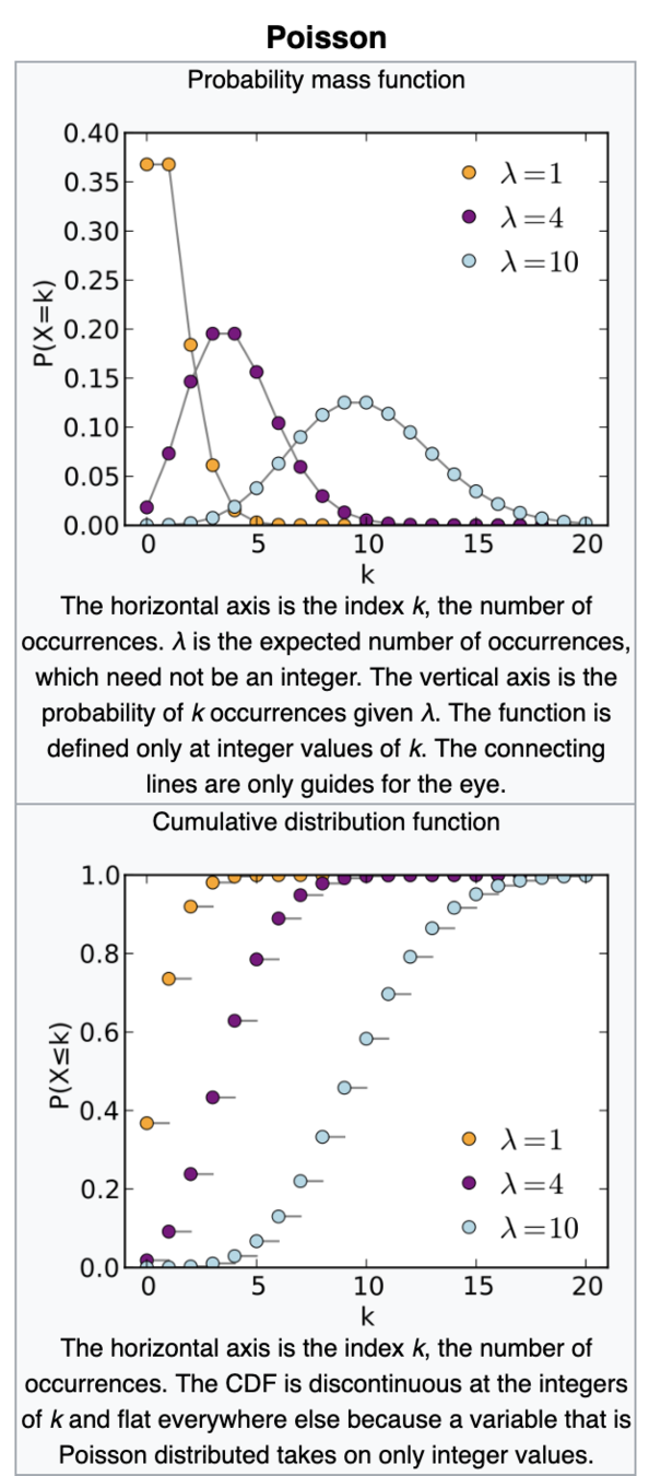
Shut noise/count noise
The innate noise in natural steady state processes (star flux, rain drops...)
λ=mean
Poisson
λ=variance
Shut noise/count noise
The innate noise in natural steady state processes (star flux, rain drops...)
Poisson
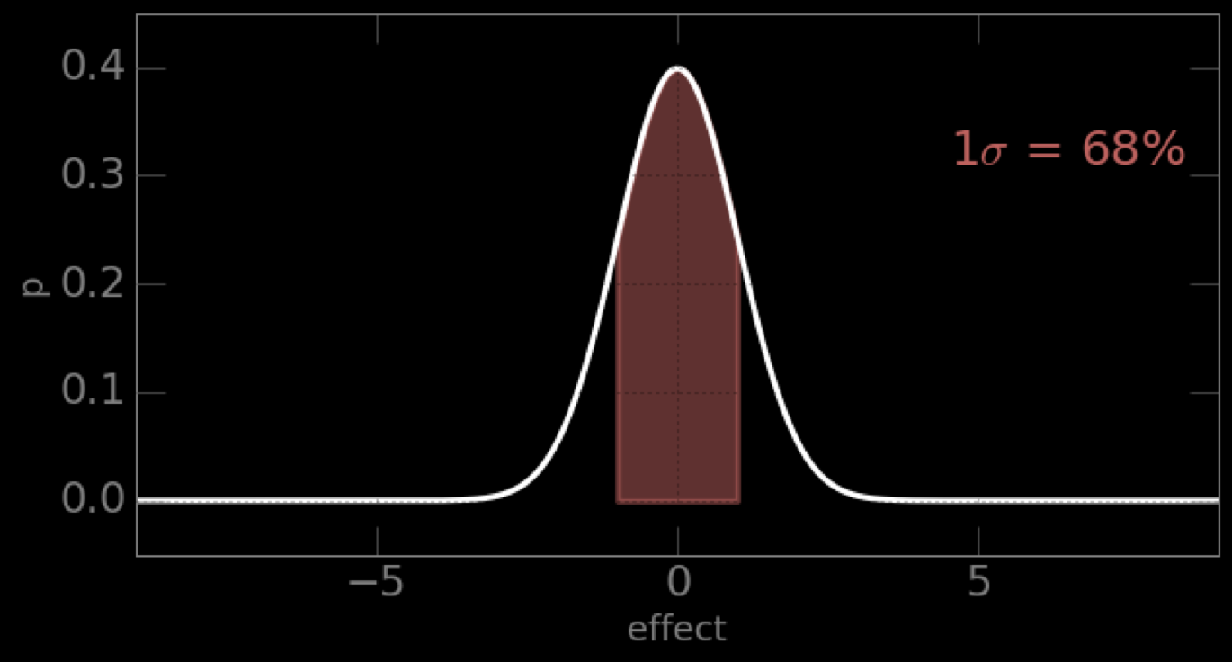
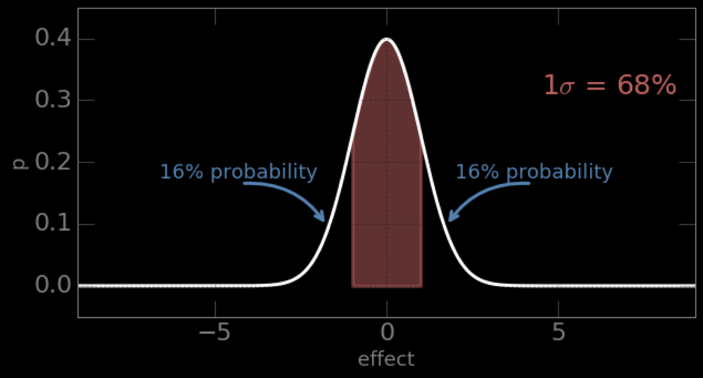
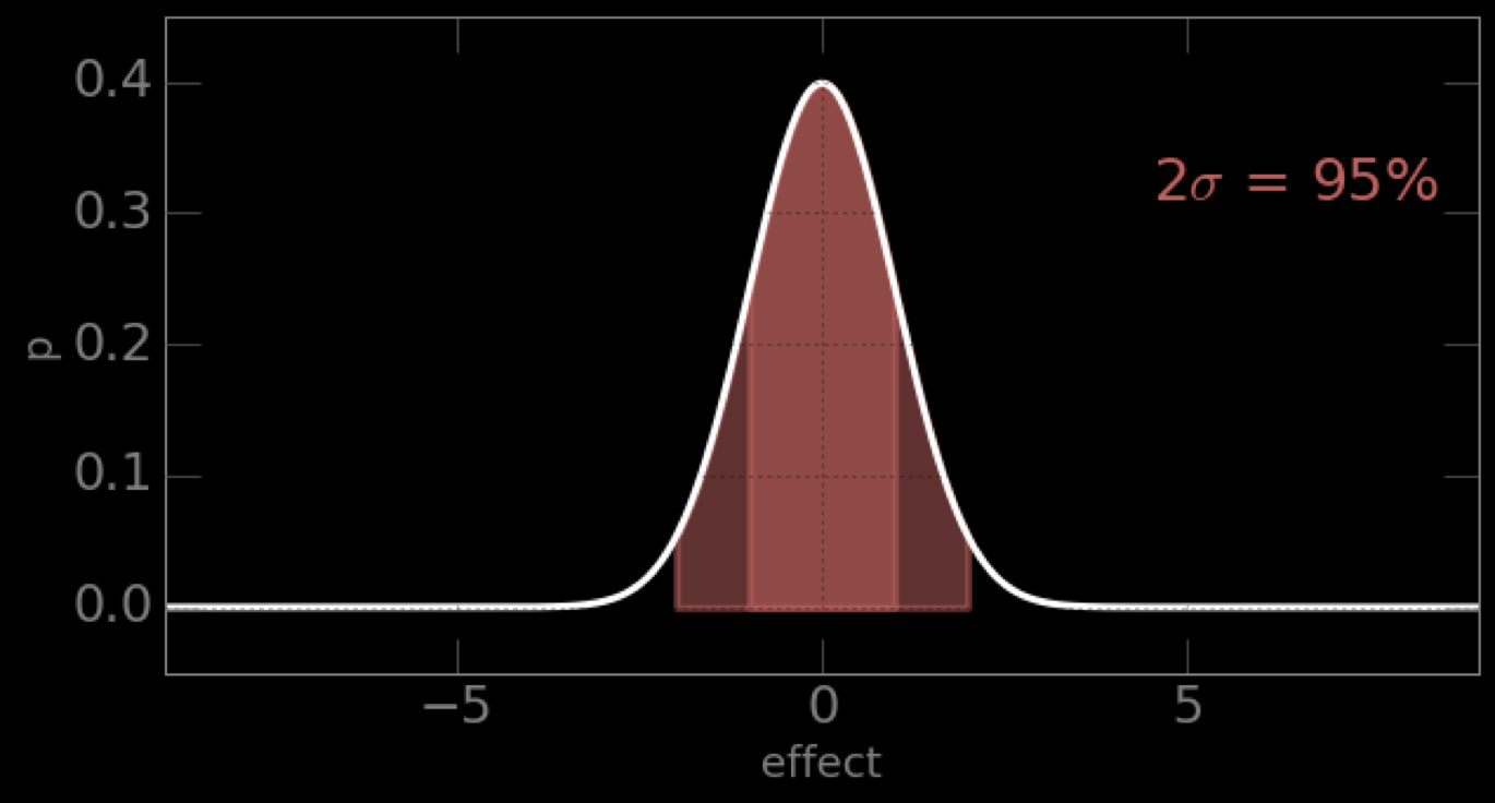
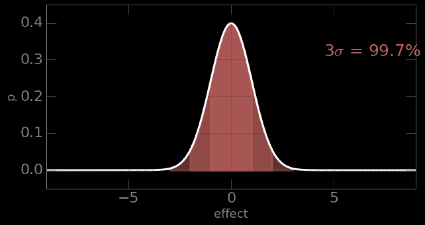
most common noise:
well behaved mathematically, symmetric, when we can we will assume our uncertainties are Gaussian distributed
Gaussian
turns out its extremely common
many pivotal quantities follow this distribution and thus many tests are based on this
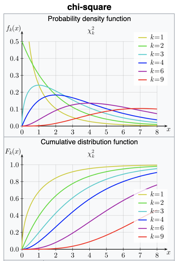
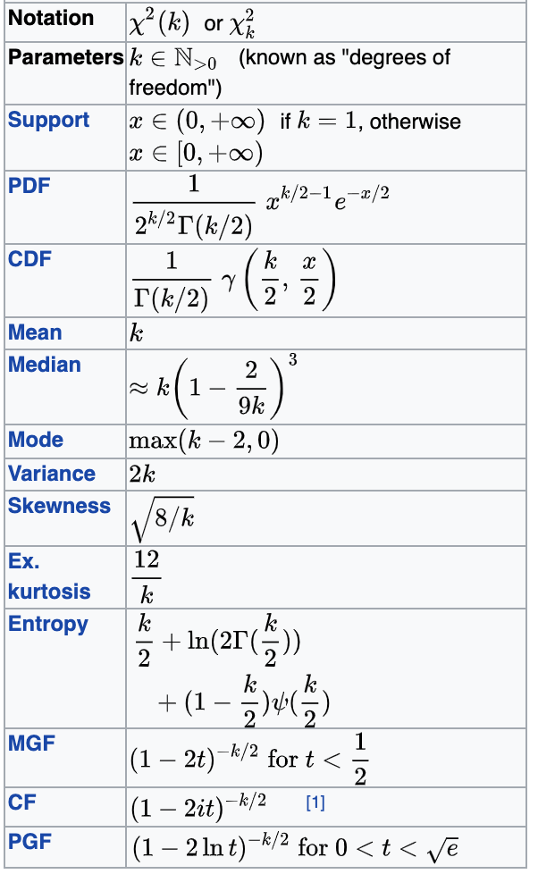
Chi-square (χ2)
By federica bianco
Foundations of Data Science for Everyone - Probability and Statistics


