


federica bianco PRO
astro | data science | data for good
Federica Bianco
University of Delaware
Rubin Observatory
dimensionality reduction - why
1/6
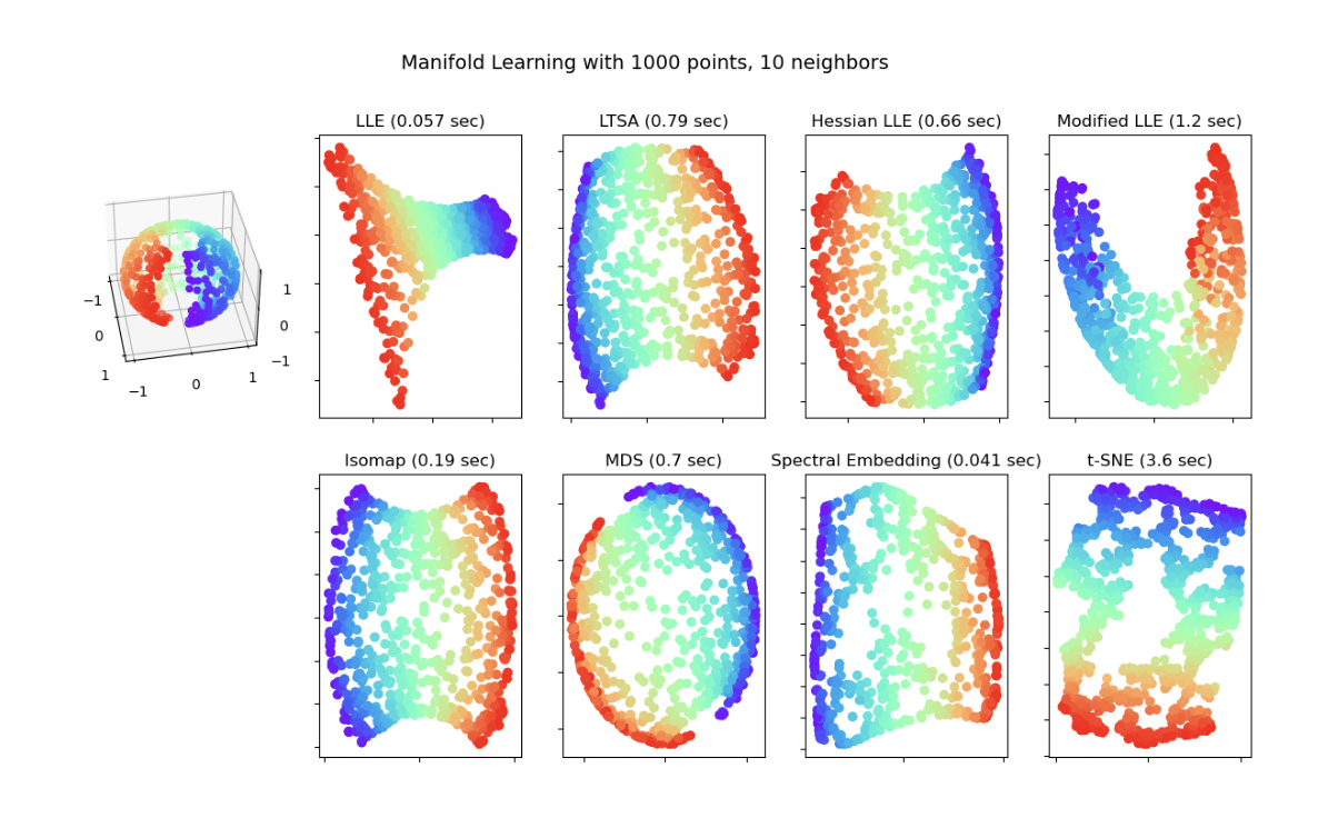
manifold lerning
2/6
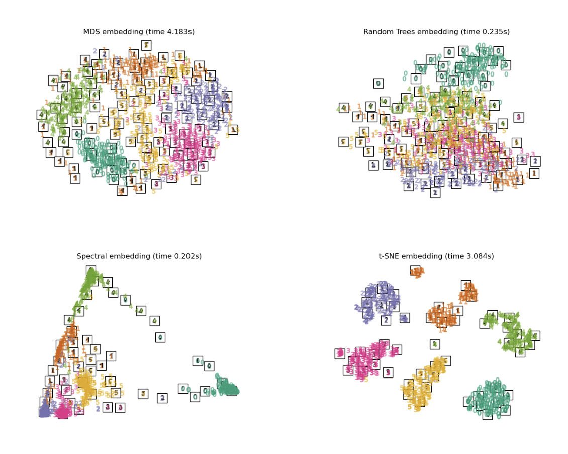
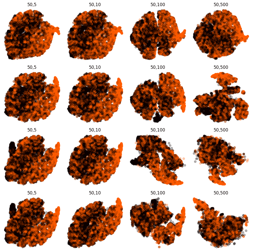
MANIFOLD LEARNING ON MNIST
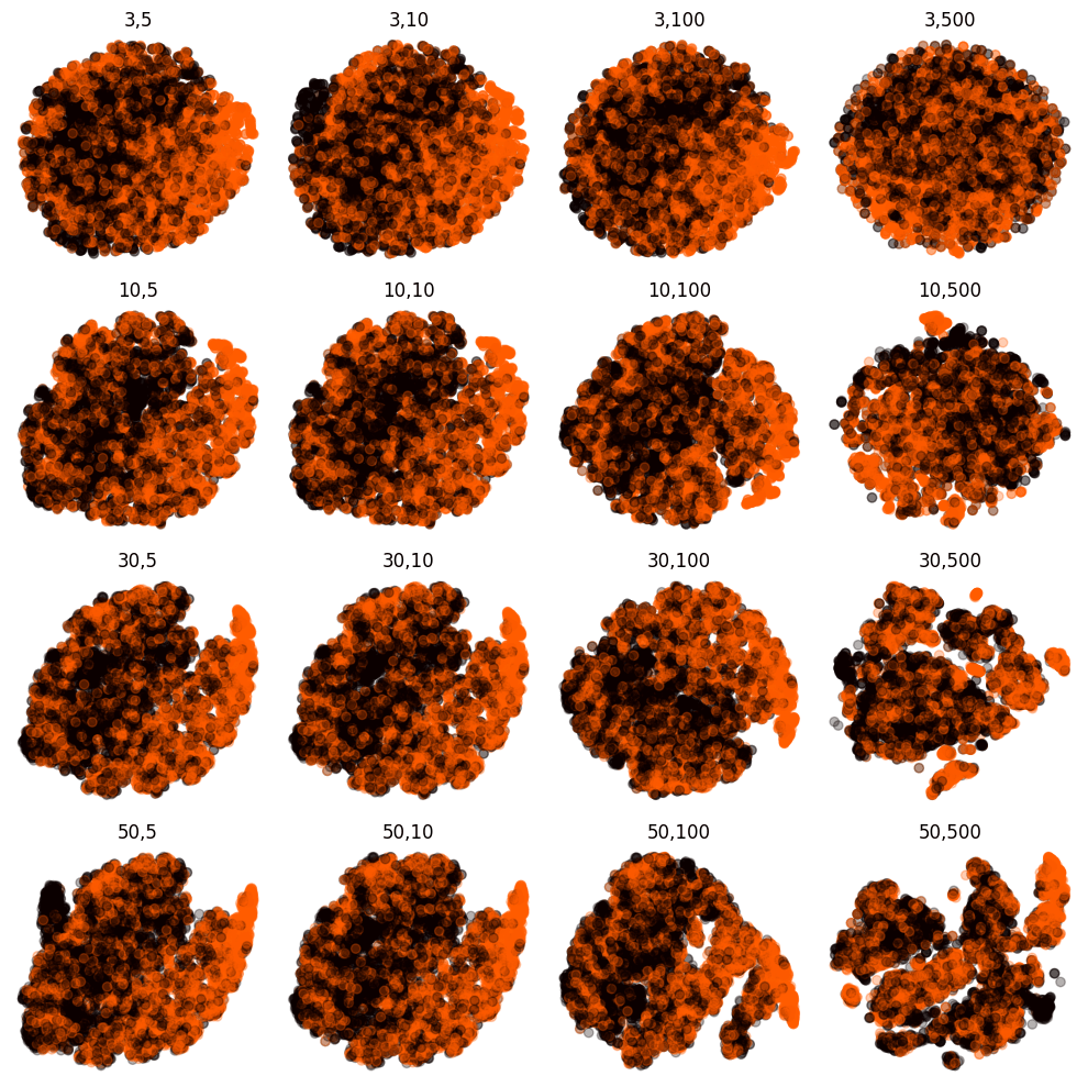
perplexity, early exaggeration
Higgs boson Kaggle dataset Training set of 250000 events, with an ID column, 30 feature columns, a weight column and a label column.
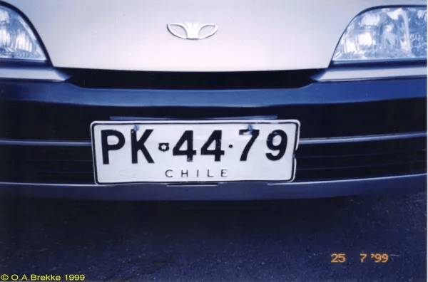
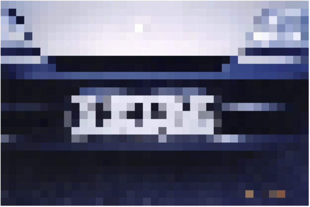
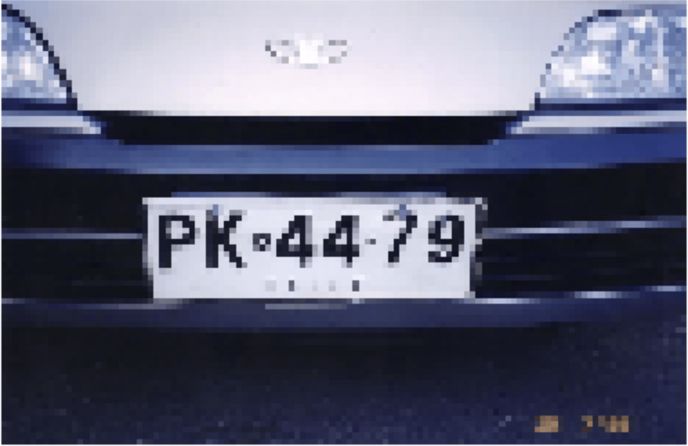
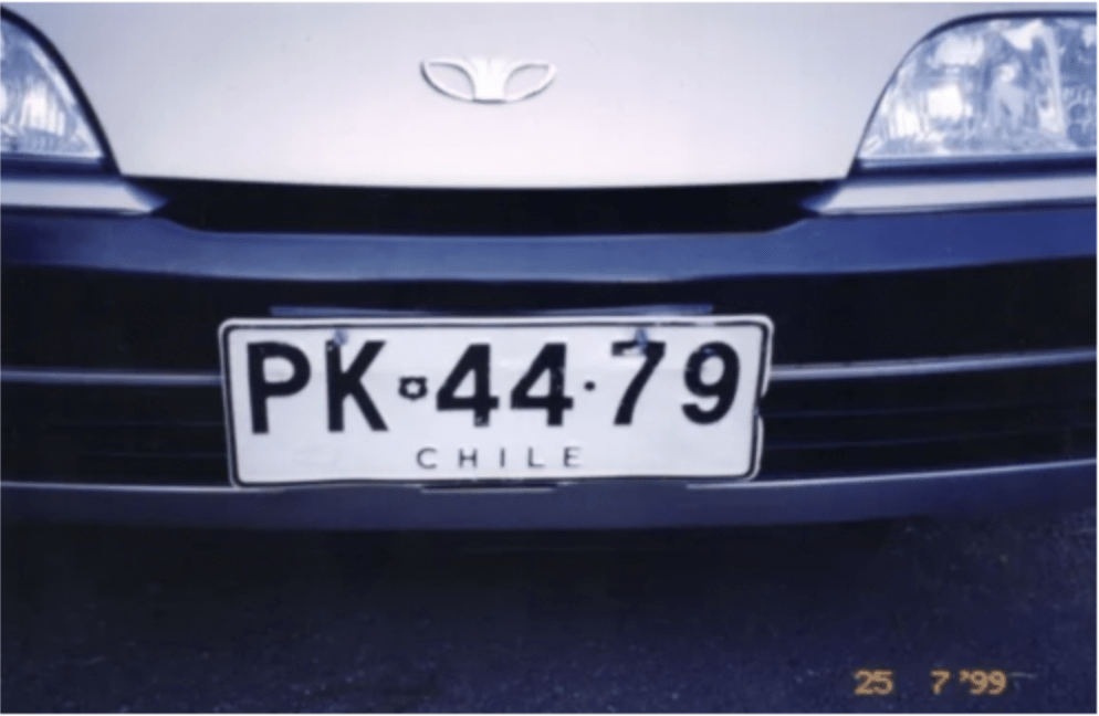
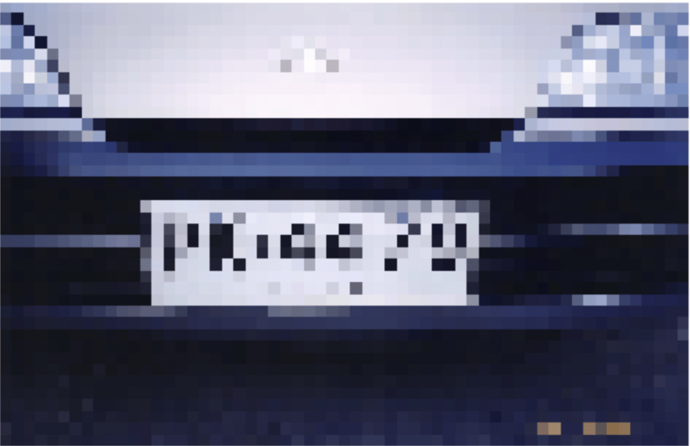
Super resolution in society and astronomy
3/6
Theory driven | Falsifiability
Experiment driven
Simulations | Probabilistic inference | Computation
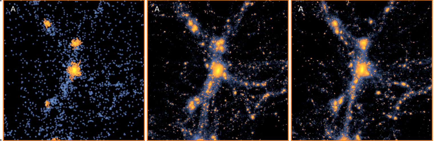
The Millennium Run used more than 10^10 particles to trace the evolution of the matter distribution in a cubic region of the Universe 500/h Mpc on a side (~over 2 billion light-years on a side), and has a spatial resolution of 5/h kpc. ~20M galaxies.
350 000 processor hours of CPU time, or 28 days of wall-clock time. Springel+2005
LOW RES SIM
HIGH RES SIM
LOW RES SIM
HIGH RES SIM
AI-AIDED HIGH RES
LOW RES SIM
HIGH RES SIM
AI-AIDED HIGH RES
INPUT
OUTPUT
TARGET
loss = D(OUTPUT-TARGET)
AUTOENCODERS
4/6
Unsupervised learning with
Neural Networks
}
5dim representation
4dim
3dim
complex imput data
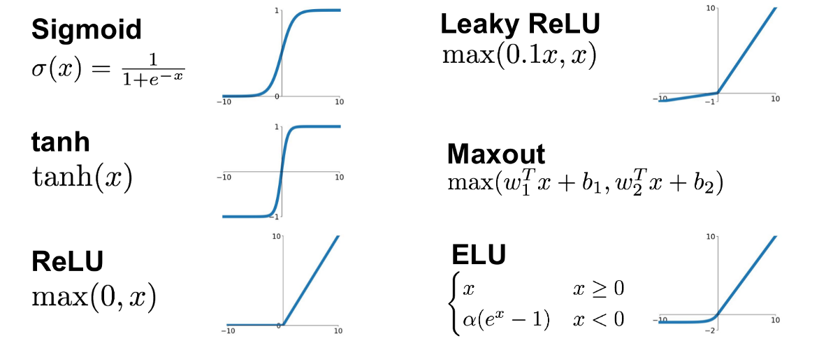
What do NN do? approximate complex functions with series of modified linear functions
Perceptrons are linear classifiers: makes its predictions based on a linear predictor function
combining a set of weights (=parameters) with the feature vector.
.
.
.
output
activation function
weights
bias
output
Fully connected: all nodes go to all nodes of the next layer.
input layer
hidden layer
output layer
1970: multilayer perceptron architecture
output
Fully connected: all nodes go to all nodes of the next layer.
layer of perceptrons
Unsupervised learning with
Neural Networks
What do NN do? approximate complex functions with series of modified linear functions
To do that they extract information from the data: each layer of the DNN produces a representation of the data a "latent representation"
}
5dim representation
4dim
3dim
complex imput data
Unsupervised learning with
Neural Networks
What do NN do? approximate complex functions with series of modified linear functions
To do that they extract information from the data: each layer of the DNN produces a representation of the data a "latent representation"
The dimensionality of that latent representation is determined by the size of the layer
.... so if my layers are smaller what I have is a compact representation of the data
}
5dim representation
4dim
3dim
complex imput data
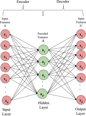
Autoencoder Architecture
Feed Forward DNN:
the size of the input is 5,
the size of the last layer is 2
Autoencoder Architecture
Feed Forward DNN:
the size of the input is 5,
the size of the last layer is 2
p(letter)
p(digit)
Autoencoder Architecture
Feed Forward DNN:
the size of the input is N,
the size of the last layer is N
Autoencoder Architecture
Feed Forward DNN:
the size of the input is <N,
the size of the last layer is N
Feed Forward DNN:
the size of the input is N,
the size of the last layer is N
Autoencoder Architecture
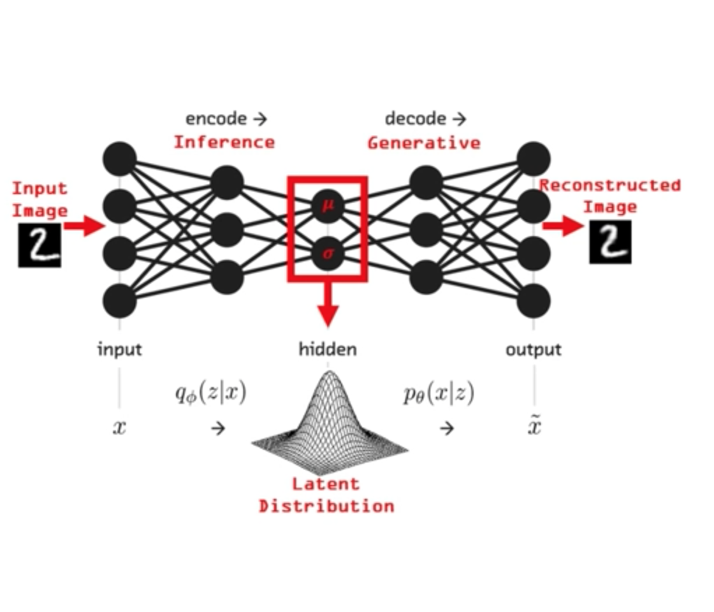
Variational Autoencoder Architecture
The hidden representation is assumed (forced) to be Gaussian. The bottle-neck layer represents the mean and standard deviation of that distribution
Building a DNN
with keras and tensorflow
Trivial to build, but the devil is in the details!
Building a DNN
with keras and tensorflow
Trivial to build, but the devil is in the details!
from keras.models import Sequential
#can upload pretrained models from keras.models
from keras.layers import Dense, Conv2D, MaxPooling2D
#create model
model = Sequential()
#create the model architecture by adding model layers
model.add(Dense(10, activation='relu', input_shape=(n_cols,)))
model.add(Dense(10, activation='relu'))
model.add(Dense(1))
#need to choose the loss function, metric, optimization scheme
model.compile(optimizer='adam', loss='mean_squared_error')
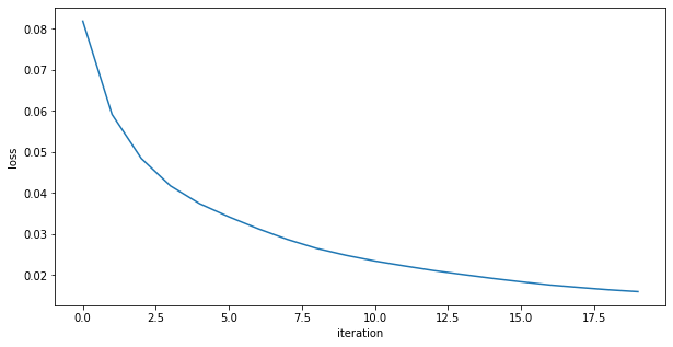
#need to learn what to look for - always plot the loss function!
model.fit(x_train, y_train, validation_data=(x_test, y_test),
epochs=20, batch_size=100, verbose=1)
#note that the model allows to give a validation test,
#this is for a 3fold cross valiation: train-validate-test
#predict
test_y_predictions = model.predict(validate_X)Building a DNN
with keras and tensorflow
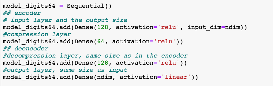
autoencoder for image recontstruction
encoder
This autoencoder model has a 64-neuron bottle neck. This means it will generate a compressed representation of the data out of that layer which is 16-dimensional (the original size is 784 pixels)
Building a DNN
with keras and tensorflow
autoencoder for image recontstruction
decoder
This autoencoder model has a 64-neuron bottle neck. This means it will generate a compressed representation of the data out of that layer which is 16-dimensional (the original size is 784 pixels)
Building a DNN
with keras and tensorflow
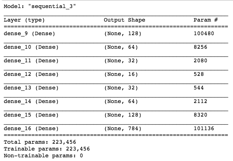
autoencoder for image recontstruction
This autoencoder model has a 64-neuron bottle neck. This means it will generate a compressed representation of the data out of that layer which is 16-dimensional (the original size is 784 pixels)
bottle neck
Building a DNN
with keras and tensorflow
autoencoder for image recontstruction
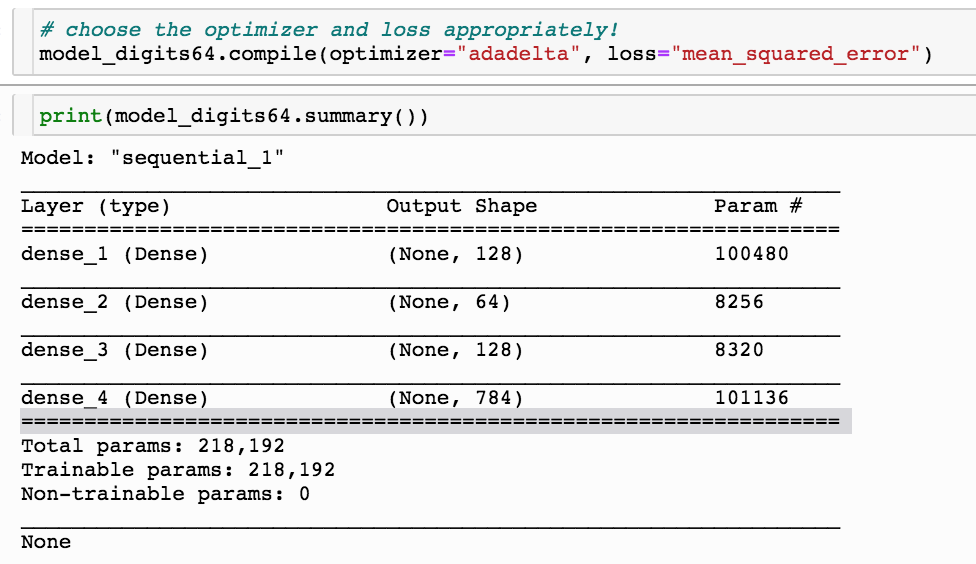
This simple model has 200K parameters!
My original choice is to train it with "adadelta" with a mean squared loss function, all activation functions are relu, appropriate for a linear regression
Building a DNN
with keras and tensorflow
autoencoder for image recontstruction
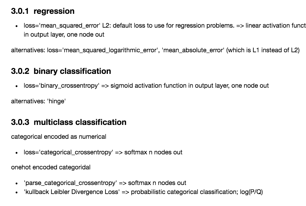
What should I choose for the loss function and how does that relate to the activation functiom and optimization?
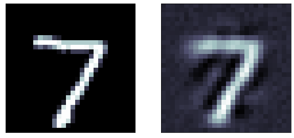
autoencoder for image recontstruction
model_digits64.add(Dense(ndim,
                        activation='linear'))
model_digits64_sig.compile(optimizer="adadelta",
                   loss="mean_squared_error")
model_digits64_sig.add(Dense(ndim,
activation='sigmoid'))
model_digits64_sig.compile(optimizer="adadelta",
loss="mean_squared_error")
model_digits64_sig.add(Dense(ndim,
activation='sigmoid'))
model_digits64_bce.compile(optimizer="adadelta",
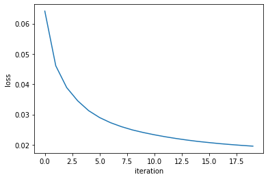
loss="binary_crossentropy")loss function: did not finish learning, it is still decreasing rapidly
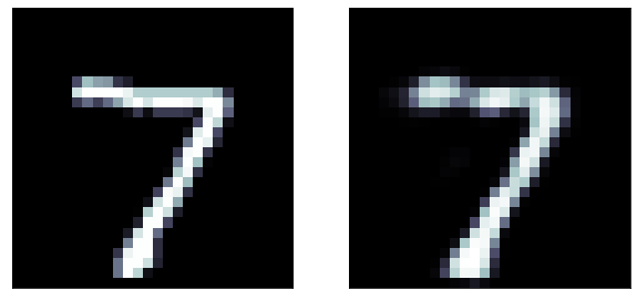
The predictions are far too detailed. While the input is not binary, it does not have a lot of details. Maybe approaching it as a binary problem (with a sigmoid and a binary cross entropy loss) will give better results
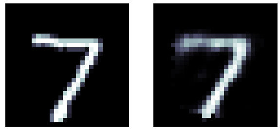
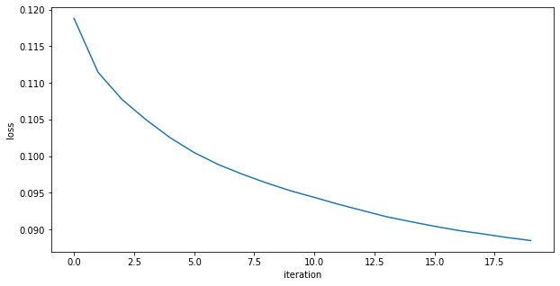
loss function: also did not finish learning, it is still decreasing rapidly
A sigmoid gives activation gives a much better result!
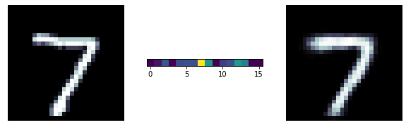
Binary cross entropy loss function: It is more appriopriate when the output layer is sigmoid
Even better results!
original
predicted
predicted
original
predicted
original
predicted
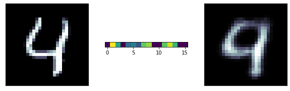
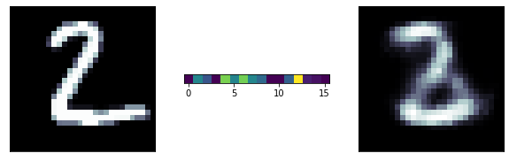
autoencoder for image recontstruction
A more ambitious model has a 16 neurons bottle neck: we are trying to extract 16 numbers to reconstruct the entire image! its pretty remarcable! those 16 number are extracted features from the data
predicted
original
latent
representation
convolution
5/6
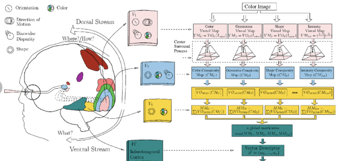
@akumadog
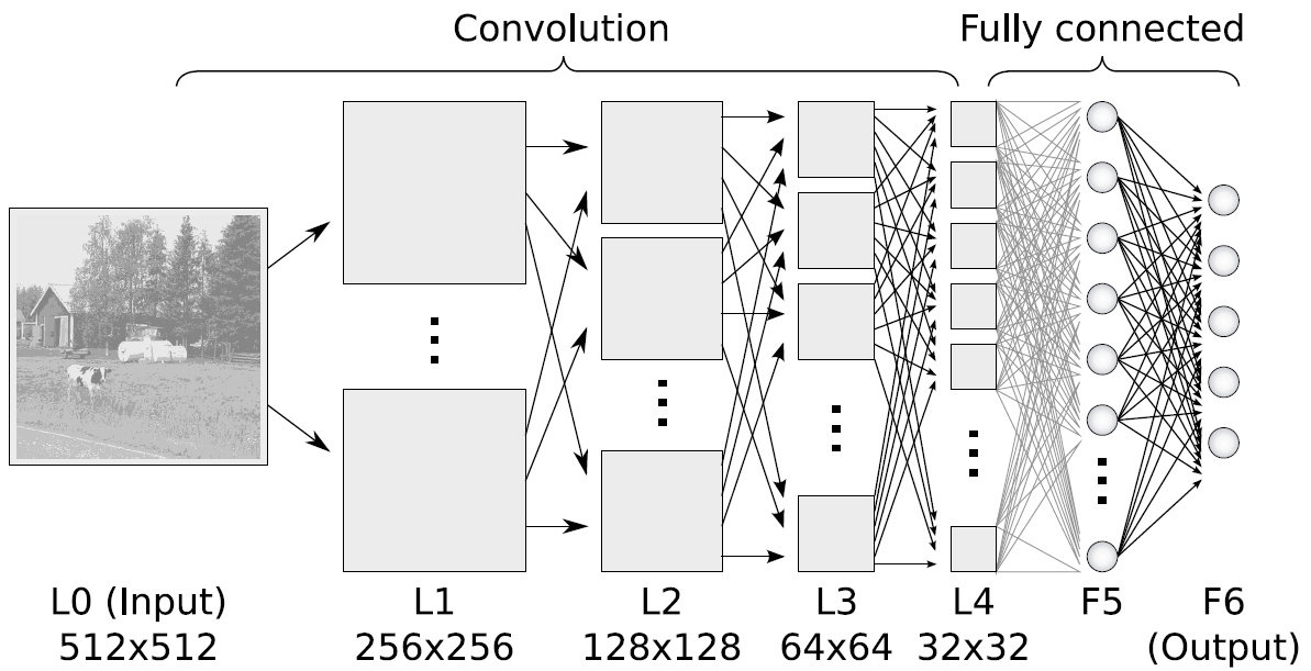
The visual cortex learns hierarchically: first detects simple features, then more complex features and ensembles of features
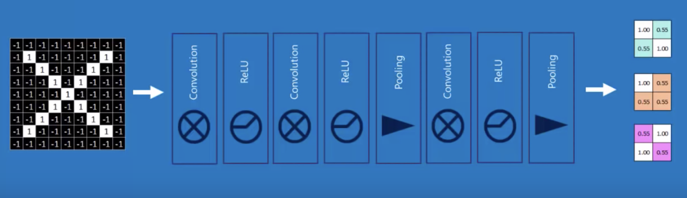
Convolution
Convolution
convolution is a mathematical operator on two functions
f and g
that produces a third function
f x g
expressing how the shape of one is modified by the other.
o
Convolution Theorem
fourier transform
two images.
model.add(Conv2D(64, kernel_size=(3, 3), activation='relu'))
| -1 | -1 | -1 | -1 | -1 |
|---|---|---|---|---|
| -1 | -1 | -1 | ||
| -1 | -1 | -1 | -1 | |
| -1 | -1 | -1 | ||
| -1 | -1 | -1 | -1 | -1 |
1
1
1
1
1
1
1
1
1
| -1 | -1 | -1 | -1 | -1 |
|---|---|---|---|---|
| -1 | -1 | -1 | -1 | -1 |
| -1 | -1 | -1 | -1 | -1 |
| -1 | -1 | -1 | -1 | -1 |
| -1 | -1 | -1 | -1 | -1 |
model.add(Conv2D(64, kernel_size=(3, 3), activation='relu'))
| 1 | -1 | -1 |
| -1 | 1 | -1 |
| -1 | -1 | 1 |
1
1
1
1
1
| -1 | -1 | -1 | -1 | -1 |
|---|---|---|---|---|
| -1 | -1 | -1 | ||
| -1 | -1 | -1 | -1 | |
| -1 | -1 | -1 | ||
| -1 | -1 | -1 | -1 | -1 |
| -1 | -1 | 1 |
| -1 | 1 | -1 |
| 1 | -1 | -1 |
feature maps
model.add(Conv2D(64, kernel_size=(3, 3), activation='relu'))
1
1
1
1
1
convolution
| -1 | -1 | -1 | -1 | -1 |
|---|---|---|---|---|
| -1 | -1 | -1 | ||
| -1 | -1 | -1 | -1 | |
| -1 | -1 | -1 | ||
| -1 | -1 | -1 | -1 | -1 |
| 1 | -1 | -1 |
| -1 | 1 | -1 |
| -1 | -1 | 1 |
model.add(Conv2D(64, kernel_size=(3, 3), activation='relu'))
1
1
1
1
1
| -1 | -1 | -1 | -1 | -1 |
|---|---|---|---|---|
| -1 | -1 | -1 | ||
| -1 | -1 | -1 | -1 | |
| -1 | -1 | -1 | ||
| -1 | -1 | -1 | -1 | -1 |
| 1 | -1 | -1 |
| -1 | 1 | -1 |
| -1 | -1 | 1 |
| 1 | -1 | -1 |
| -1 | 1 | -1 |
| -1 | -1 | 1 |
| 7 | ||
|---|---|---|
=
model.add(Conv2D(64, kernel_size=(3, 3), activation='relu'))
1
1
1
1
1
| -1 | -1 | -1 | -1 | -1 |
|---|---|---|---|---|
| -1 | -1 | -1 | ||
| -1 | -1 | -1 | -1 | |
| -1 | -1 | -1 | ||
| -1 | -1 | -1 | -1 | -1 |
| 1 | -1 | -1 |
| -1 | 1 | -1 |
| -1 | -1 | 1 |
| 1 | -1 | -1 |
| -1 | 1 | -1 |
| -1 | -1 | 1 |
| 7 | -3 | |
|---|---|---|
=
model.add(Conv2D(64, kernel_size=(3, 3), activation='relu'))
1
1
1
1
1
| -1 | -1 | -1 | -1 | -1 |
|---|---|---|---|---|
| -1 | -1 | -1 | ||
| -1 | -1 | -1 | -1 | |
| -1 | -1 | -1 | ||
| -1 | -1 | -1 | -1 | -1 |
| 1 | -1 | -1 |
| -1 | 1 | -1 |
| -1 | -1 | 1 |
| 1 | -1 | -1 |
| -1 | 1 | -1 |
| -1 | -1 | 1 |
| 7 | -3 | 3 |
|---|---|---|
=
model.add(Conv2D(64, kernel_size=(3, 3), activation='relu'))
1
1
1
1
1
| -1 | -1 | -1 | -1 | -1 |
|---|---|---|---|---|
| -1 | -1 | -1 | ||
| -1 | -1 | -1 | -1 | |
| -1 | -1 | -1 | ||
| -1 | -1 | -1 | -1 | -1 |
| 1 | -1 | -1 |
| -1 | 1 | -1 |
| -1 | -1 | 1 |
| 1 | -1 | -1 |
| -1 | 1 | -1 |
| -1 | -1 | 1 |
| 7 | -1 | 3 |
|---|---|---|
| ? | ||
=
model.add(Conv2D(64, kernel_size=(3, 3), activation='relu'))
1
1
1
1
1
| -1 | -1 | -1 | -1 | -1 |
|---|---|---|---|---|
| -1 | -1 | -1 | ||
| -1 | -1 | -1 | -1 | |
| -1 | -1 | -1 | ||
| -1 | -1 | -1 | -1 | -1 |
| 1 | -1 | -1 |
| -1 | 1 | -1 |
| -1 | -1 | 1 |
| 1 | -1 | -1 |
| -1 | 1 | -1 |
| -1 | -1 | 1 |
| 7 | -1 | 3 |
|---|---|---|
| ? | ? | |
=
model.add(Conv2D(64, kernel_size=(3, 3), activation='relu'))
1
1
1
1
1
| -1 | -1 | -1 | -1 | -1 |
|---|---|---|---|---|
| -1 | -1 | -1 | ||
| -1 | -1 | -1 | -1 | |
| -1 | -1 | -1 | ||
| -1 | -1 | -1 | -1 | -1 |
| 1 | -1 | -1 |
| -1 | 1 | -1 |
| -1 | -1 | 1 |
| 7 | -1 | 3 |
|---|---|---|
| -3 | ||
=
input layer
feature map
convolution layer
model.add(Conv2D(64, kernel_size=(3, 3), activation='relu'))
1
1
1
1
1
| -1 | -1 | -1 | -1 | -1 |
|---|---|---|---|---|
| -1 | -1 | -1 | ||
| -1 | -1 | -1 | -1 | |
| -1 | -1 | -1 | ||
| -1 | -1 | -1 | -1 | -1 |
| 1 | -1 | -1 |
| -1 | 1 | -1 |
| -1 | -1 | 1 |
| 7 | -3 | 3 |
| -3 | 5 | -3 |
| 3 | -1 | 7 |
=
input layer
feature map
convolution layer
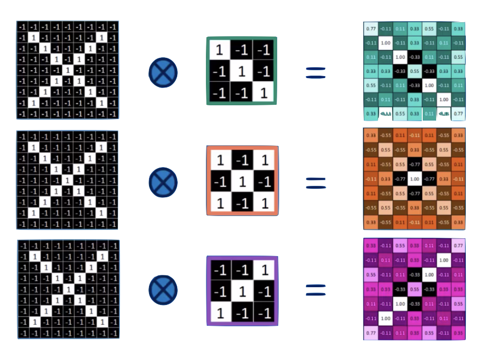
the feature map is "richer": we went from binary to R
model.add(Conv2D(64, kernel_size=(3, 3), activation='relu'))
1
1
1
1
1
| -1 | -1 | -1 | -1 | -1 |
|---|---|---|---|---|
| -1 | -1 | -1 | ||
| -1 | -1 | -1 | -1 | |
| -1 | -1 | -1 | ||
| -1 | -1 | -1 | -1 | -1 |
| 1 | -1 | -1 |
| -1 | 1 | -1 |
| -1 | -1 | 1 |
| 7 | -3 | 3 |
| -3 | 5 | -3 |
| 3 | -1 | 7 |
=
input layer
feature map
convolution layer
the feature map is "richer": we went from binary to R
and it is reminiscent of the original layer
7
5
7
model.add(Conv2D(64, kernel_size=(3, 3), activation='relu'))
Convolve with different feature: each neuron is 1 feature
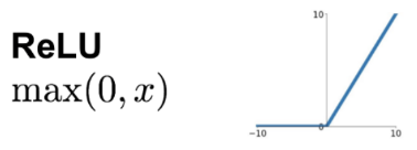
ReLu
| 7 | -3 | 3 |
| -3 | 5 | -3 |
| 3 | -1 | 7 |
7
5
7
ReLu: normalization that replaces negative values with 0's
| 7 | 0 | 3 |
| 0 | 5 | 0 |
| 3 | 0 | 7 |
7
5
7
model.add(Conv2D(64, kernel_size=(3, 3), activation='relu'))
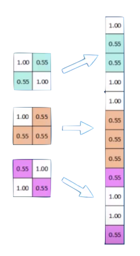
Max-Pool
MaxPooling: reduce image size, generalizes result
| 7 | 0 | 3 |
| 0 | 5 | 0 |
| 0 | 0 | 7 |
7
5
7
MaxPooling: reduce image size, generalizes result
| 7 | 0 | 3 |
| 0 | 5 | 0 |
| 3 | 0 | 7 |
7
5
7
2x2 Max Poll
| 7 | 5 |
MaxPooling: reduce image size, generalizes result
| 7 | 0 | 3 |
| 0 | 5 | 0 |
| 3 | 0 | 7 |
7
5
7
2x2 Max Poll
| 7 | 5 |
| 5 |
MaxPooling: reduce image size, generalizes result
| 7 | 0 | 3 |
| 0 | 5 | 0 |
| 3 | 0 | 7 |
7
5
7
2x2 Max Poll
| 7 | 5 |
| 5 | 7 |
MaxPooling: reduce image size & generalizes result
By reducing the size and picking the maximum of a sub-region we make the network less sensitive to specific details
model.add(MaxPooling2D(pool_size=(2, 2)))from keras.models import Sequential
from keras.layers import Dense, Dropout, Flatten
from keras.layers import Conv2D, MaxPooling2D
model = Sequencial()
model.add(Conv2D(32, kernel_size=(10, 10),
activation='relu',
input_shape=input_shape))
model.add(Conv2D(64, kernel_size=(3, 3), activation='relu'))
model.add(MaxPooling2D(pool_size=(2, 2)))
model.add(Conv2D(32, kernel_size=(3, 3), activation='relu'))
model.add(MaxPooling2D(pool_size=(2, 2)))x
O
last hidden layer
output layer
from keras.models import Sequential
from keras.layers import Dense, Dropout, Flatten
from keras.layers import Conv2D, MaxPooling2D
model = Sequencial()
model.add(Conv2D(32, kernel_size=(10, 10),
                 activation='relu',
                 input_shape=input_shape))
model.add(Conv2D(64, kernel_size=(3, 3), activation='relu'))
model.add(MaxPooling2D(pool_size=(2, 2)))
model.add(Conv2D(32, kernel_size=(3, 3), activation='relu'))
model.add(MaxPooling2D(pool_size=(2, 2)))
model.add(Flatten())
model.add(Dense(128, activation='relu'))
model.add(Dense(2, activation='softmax'))Stack multiple convolution layers
Generative AI in society
6/6
White Males
White Female
Non-White Males
Non-White Female
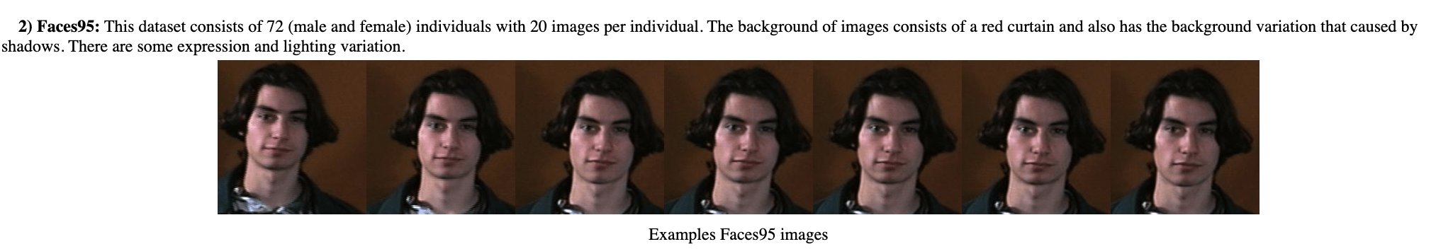
Faces95 - Computer Vision Science Research Projects, Dr Libor Spacek.
White Males: 43
White Female: 6
Non-White Males: 12
Non-White Female: 1
Faces95 - Computer Vision Science Research Projects, Dr Libor Spacek.
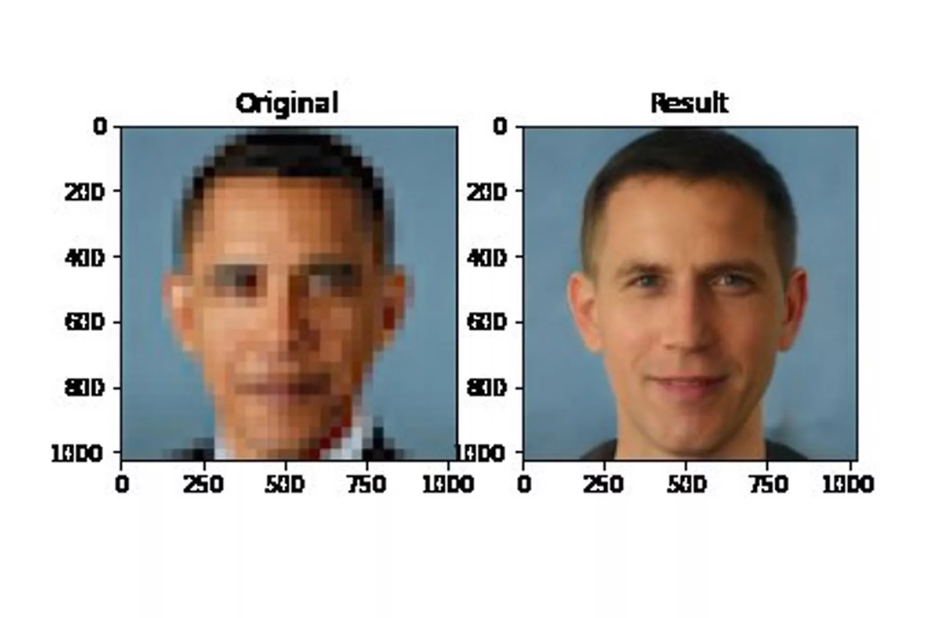
Why does this AI model whitens Obama face?
Simple answer: the data is biased. The algorithm is fed more images of white people
But really, would the opposite have been acceptable? The bias is in society
Why does this AI model whitens Obama face?
Simple answer: the data is biased. The algorithm is fed more images of white people
The bias is in the data
The bias is in the models and the decision we make
The bias is in how we choose to optimize our model
Should AI reflect
who we are
(and enforce and grow our bias)
or should it reflect who we aspire to be?
(and who decides what that is?)
The bias is society that provides the framework to validate our biased models
The bias is in the data
The bias is in the models and the decision we make
The bias is in how we choose to optimize our model
The bias is society that provides the framework to validate our biased models
none of this is new
https://www.nytimes.com/2019/04/25/lens/sarah-lewis-racial-bias-photography.html
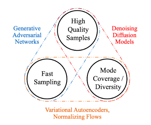
In defense of autoencoders
7/6
see also https://arxiv.org/pdf/2103.04922.pdf
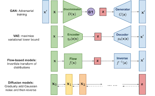
Which generative AI is right for you??
thank you!
University of Delaware
Department of Physics and Astronomy
Biden School of Public Policy and Administration
Data Science Institute
federica bianco
fbianco@udel.edu
By federica bianco


