


federica bianco PRO
astro | data science | data for good
dr.federica bianco | fbb.space | fedhere | fedhere
models - linear regression - uncertainties
this slide deck:
1
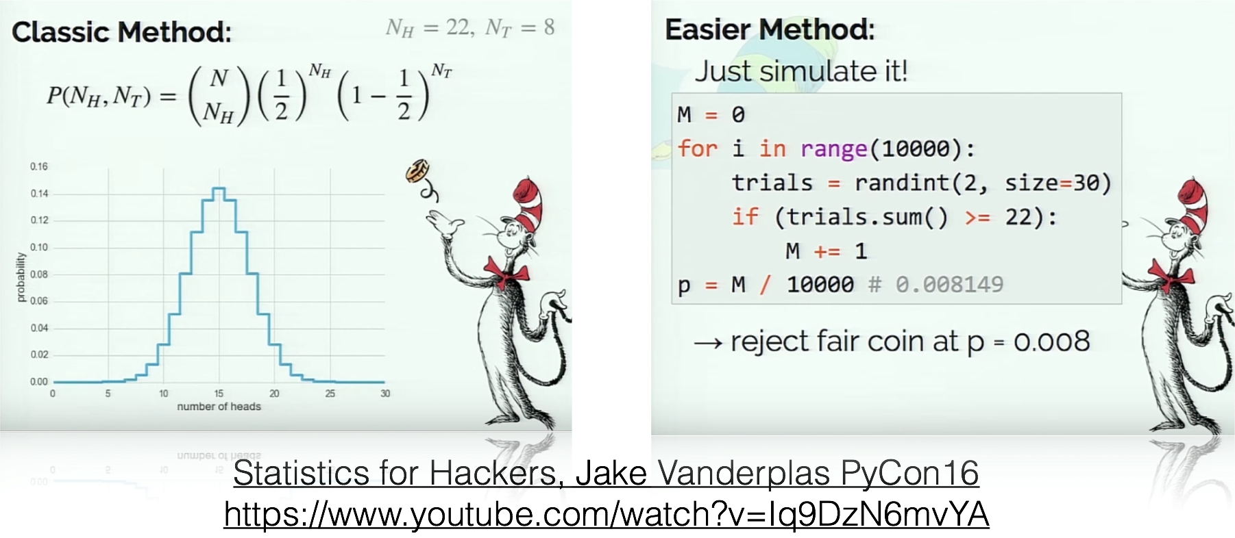
NHRT
formulate your prediction (NH)
identify all alternative outcomes (AH)
set confidence threshold
(p-value)
find a measurable quantity which under the Null has a known distribution
(pivotal quantity)
calculate the pivotal quantity
calculate probability of value obtained for the pivotal quantity under the Null
if probability < p-value : reject Null
Key Slide
Null
Hypothesis
Rejection
Testing
Alternative Hypothesis
if all alternatives to our model are ruled out, then our model must hold
identify all alternative outcomes
Null
Hypothesis
Rejection
Testing
test data against alternative outcomes
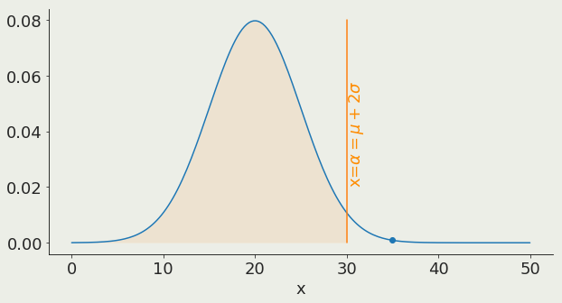
95%
α is the x value corresponding to a chosen threshold
it represent the probability to get a result at least as extreme just by chance
1
[Machine Learning is the] field of study that gives computers the ability to learn without being explicitly programmed.
Arthur Samuel, 1959
[Machine Learning is the] field of study that gives computers the ability to learn without being explicitly programmed.
Arthur Samuel, 1959
model
parameters: slope (a), intercept (b)
Model:
a mathematical formula with parameters
Model:
a mathematical formula with parameters
[Machine Learning is the] field of study that gives computers the ability to learn without being explicitly programmed.
Arthur Samuel, 1959
model variable: x - for example time, location, energy
model
parameters: slope (a), intercept (b)
Model:
a mathematical formula with parameters
[Machine Learning is the] field of study that gives computers the ability to learn without being explicitly programmed.
Arthur Samuel, 1959
model variable: x - for example time, location, energy
model
Data:
a set of observations
Model:
a mathematical formula with parameters
[Machine Learning is the] field of study that gives computers the ability to learn without being explicitly programmed.
Arthur Samuel, 1959
[Machine Learning is the] field of study that gives computers the ability to learn without being explicitly programmed.
Arthur Samuel, 1959
Data:
a set of observations
Model:
a mathematical formula with parameters
for every parameter there are an infinity of models
[Machine Learning is the] field of study that gives computers the ability to learn without being explicitly programmed.
Arthur Samuel, 1959
Data:
a set of observations
Model:
a mathematical formula with parameters
Use the data to learn the parameters of the model
Machine Learning models are parametrized representation of "reality" where the parameters are learned from finite sets of realizations of that reality
Machine Learning is the disciplines that conceptualizes, studies, and applies those models.
Key Concept
Use the data to learn the parameters of the model
the best way to think about it in the ML context:
a model is a low dimensional representation of a higher dimensionality dataset
1.2
used to:
Clustering
partitioning the feature space so that the existing data is grouped (according to some target function!)
Clustering
partitioning the feature space so that the existing data is grouped (according to some target function!)
Unsupervised learning
All features are observed for all datapoints
Clustering
partitioning the feature space so that the existing data is grouped (according to some target function!)
Classifying & regression
finding functions of the variables that allow to predict unobserved properties of new observations
Unsupervised learning
Supervised learning
All features are observed for all datapoints
Some features are not observed for some data points we want to predict them.
Unsupervised learning
Supervised learning
All features are observed for all datapoints
and we are looking for structure in the feature space
Some features are not observed for some data points we want to predict them.
The datapoints for which the target feature is observed are said to be "labeled"
Semi-supervised learning
Active learning
A small amount of labeled data is available. Data is cluster and clusters inherit labels
The code can interact with the user to update labels.
also...
1.3
How do we measure if a model is good?
Accuracy
Precision
Recall
ROC
AOC
We will talk more about this later...
but for now focus on
regression performance metrics
How do we measure if a model is good?
Accuracy
Precision
Recall
ROC
AOC
Absolute error
Squared error
Mean squared error
Root mean
squared error
Relative mean
squared error
R squared
We will talk more about this later...
but for now focus on
regression performance metrics
How do we measure if a model is good?
Accuracy
Precision
Recall
ROC
AOC
Absolute error
Squared error
Mean squared error
Root mean
squared error
Relative mean
squared error
R squared
do you recognize these??
We will talk more about this later...
but for now focus on
regression performance metrics
How do we measure if a model is good?
Accuracy
Precision
Recall
ROC
AOC
We will talk more about this later...
but for now focus on
regression performance metrics
Absolute error
Squared error
Mean squared error
Root mean
squared error
Relative mean
squared error
R squared
How do we measure if a model is good?
Accuracy
Precision
Recall
ROC
AOC
We will talk more about this later...
but for now focus on
regression performance metrics
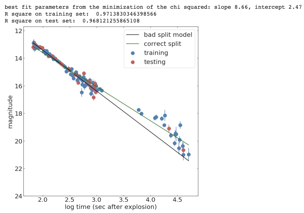
Split the sample in test and training sets
Train on the training set
Test (measure accuracy) on the test set
from sklearn.model_selection import train_test_split

def line(x, intercept, slope):
    return slope * x + intercept

def chi2(args, x, y, s):
    a, b = args
    return sum((y - line(x, a, b))**2 / s)

x_train, x_test, y_train, y_test, s_train, s_test = train_test_split(
     x, y, s, test_size=0.25, random_state=42)

initialGuess = (10, 1)

chi2Solution_goodsplit = minimize(chi2, initialGuess,
	args=(x_train, y_train, s_train))

print("best fit parameters from the minimization of the chi squared: " +
       "slope {:.2f}, intercept {:.2f}".format(*chi2Solution_goodsplit.x))

print("R square on training set: ", Rsquare(chi2Solution_goodsplit.x, x_train, y_train))
print("R square on test set: ", Rsquare(chi2Solution_goodsplit.x, x_test, y_test))ML standard
In ML models need to be "validated":
The performance on the model is the performance achieved on the test set.
An upgrade on this workflow is to create a training, a test, and a validation test. Iterate between training and test to achieve optimal performance, then measure accuracy on the validation set.This is because you can use the test set performance to tune the model hyperparameters (model selection) but then you would report a performance that is tuned on the test set.
a significance performance degradation on the test compared to training set indicates that the model is "overtrained" and does not generalize well.
Intermission: Gamma Ray Bursts
TL;DR: Gamma-ray bursts (GRBs) are bright X-ray and gamma-ray flashes observed in the sky, emitted by distant extragalactic sources. They are associated with the creation or merging of neutron stars or black holes.
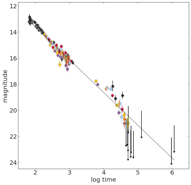
Reprocessed X- and gamma-ray emission is visible in optical wavelengths, the "afterglow"
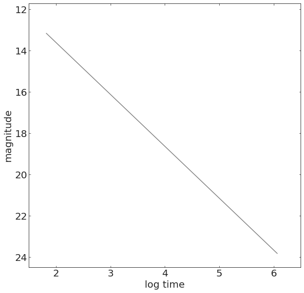
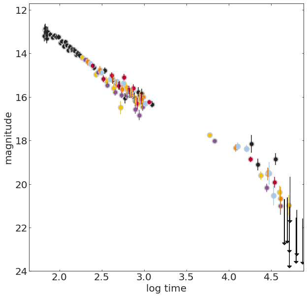
We measure a quantity named magnitude over time, which is an inverse logaritmic measure of brightness of the GRB, and which is expected to change it roughly linearly with the logarithm of time.
[ref]
Details: The light that we measure from these explosions changes over time, so we can study its time series or lightcurve.
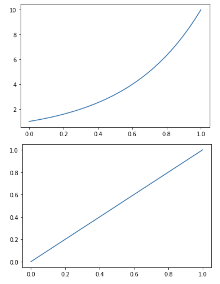
The GRB afterglow is generated by a power-law process.
The change in light follows a power law, it's not linear, but
the logarithm of a power law is a line.
The logarithm (base 10) of the light flux is called magnitude in astronomy.
m = 25 - 2.5log10(flux)
power law
x
10
x
log10(10 )
More Details: It is believed that the afterglow originates in the external shock produced as the blast wave from the explosion collides with and sweeps up material in the surrounding interstellar medium. The emission is synchrotron emission produced when electrons are accelerated in the presence of a magnetic field. The successive afterglows at progressively lower wavelengths (X-ray, optical, radio) result naturally as the expanding shock wave sweeps up more and more material causing it to slow down and lose energy.
*X-ray afterglows have been observed for all GRBs, but only about 50% of GRBs also exhibit afterglows at optical and radio wavelengths [ref]
grb050525A
2
Regression
WHY?
Fitting a line
ax+b
to data y
WHY?
Fitting a line
ax+b
to data y
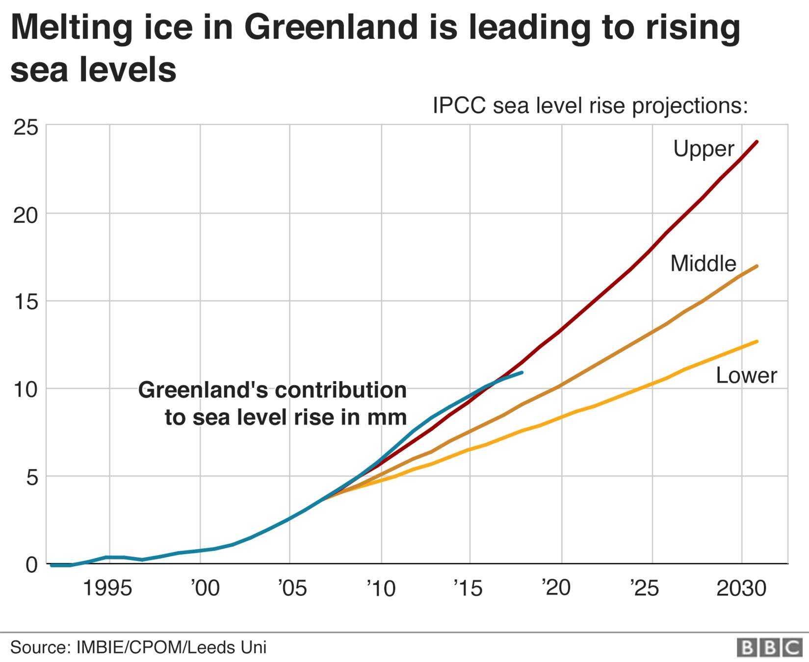
To predict and forecast
time (year)
See level contribution (mm)
Regression
To explain
distance / age of the Universe
Universe's expansion rate
supernova (stellar explosion)
measure the expansion rate at the Universe as a function of time.
Deviation from linear falsify an adiabatically expanding Universe
time (year)
WHY?
Fitting a line
ax+b
to data y
To predict and forecast
See level contribution (mm)
Regression
Key Concept
& Model Fitting
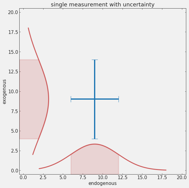
We fit models to data in order to:
Predict and forecast: predict the value of the endogenous (dependent) variable at locations of the exogenous (independent, time) variable where we have no observations. This can be within the observed range, or outside of the range, which in time-series means predict the future (forecast)
Explain: relate observed behavior to first principles or behavior of possibly variables to explain the evolution and assess causality.
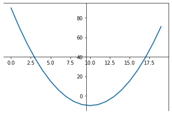
E.g. fitting a parabola to a bouncing ball demonstrates that gravity (and initial velocity) explains the behavior
Regression
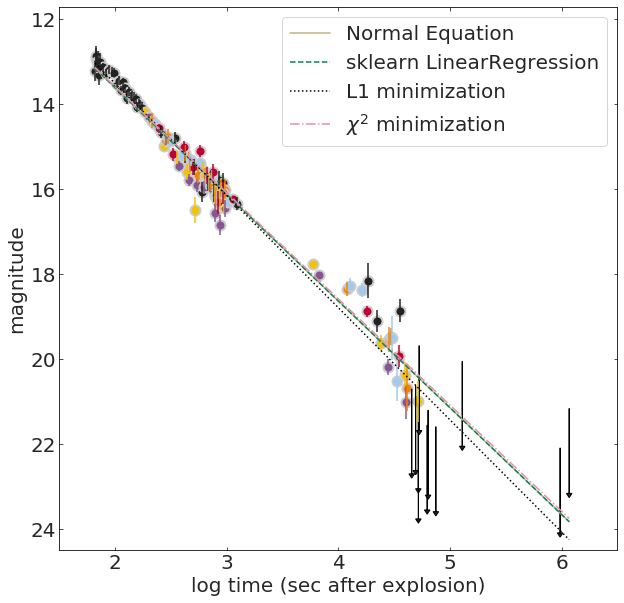
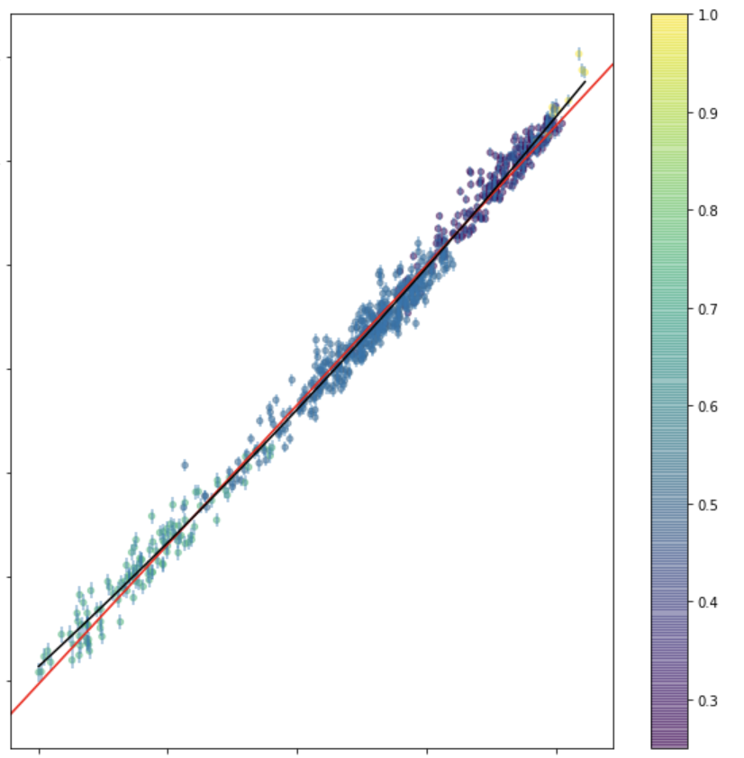
analytical solution
2.1
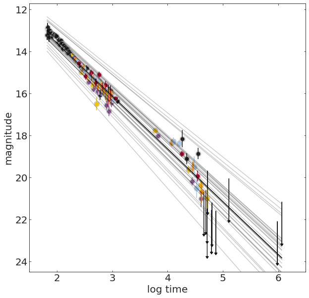
It can be shown that the optimal parameters for a line fit to data without uncertainties is:
x = grbAG[grbAG.upperlimit == 0].logtime.values
y = grbAG.loc[grbAG.upperlimit == 0].mag.values

X = np.c_[np.ones((len(x), 1)), x]


theta_best = np.linalg.inv(X.T.dot(X)).dot(X.T).dot(y)It can be shown that the optimal parameters for a line fit to data without uncertainties is:
independent variable
2x1
x = grbAG[grbAG.upperlimit == 0].logtime.values
y = grbAG.loc[grbAG.upperlimit == 0].mag.values

X = np.c_[np.ones((len(x), 1)), x]


theta_best = np.linalg.inv(X.T.dot(X)).dot(X.T).dot(y)
2xN Nx2 2xN Nx1
It can be shown that the optimal parameters for a line fit to data without uncertainties is:
from sklearn.linear_model import LinearRegression
lr = LinearRegression()

x = grbAG[grbAG.upperlimit == 0].logtime.values
y = grbAG.loc[grbAG.upperlimit == 0].mag.values

X = np.c_[np.ones((len(x), 1)), x]

lr.fit(X, y)
lr.coef_, lr.intercept_
We can let sklearn solve the equation for us:
2x1
x = grbAG[grbAG.upperlimit == 0].logtime.values
y = grbAG.loc[grbAG.upperlimit == 0].mag.values

X = np.c_[np.ones((len(x), 1)), x]


theta_best = np.linalg.inv(X.T.dot(X)).dot(X.T).dot(y)
2xN Nx2 2xN Nx1
objective function
2.2
time
time
time
time
time
time
which is the "best fit" line? A , B, C, D?
A
B
C
D
time
time
time
chi square: relates to the likelihood if the distribution is Gaussian
from scipy.optimize import minimize
def line(a, b, x):
    return a * x + b
def fitfunc(args, x, y):
    a, b = args
    return np.abs((y - line(a, b, x)))

x = grbAG[grbAG.upperlimit == 0].logtime.values
y = grbAG.loc[grbAG.upperlimit == 0].mag.values
initialGuess = (10, 1)

fitfunc(initialGuess, x, y)
solution = minimize(fitfunc, initialGuess, args=(x, y))from scipy.optimize import minimize
def line(a, b, x):
return a * x + b
def fitfunc(args, x, y):
a, b = args
return np.sum((y - line(a, b, x))**2)
x = grbAG[grbAG.upperlimit == 0].logtime.values
y = grbAG.loc[grbAG.upperlimit == 0].mag.values
initialGuess = (10, 1)
fitfunc(initialGuess, x, y)
solution = minimize(fitfunc, initialGuess, args=(x, y))from scipy.optimize import minimize
def line(a, b, x):
return a * x + b
def chi2(args, x, y, s):
a, b = args
return np.sum((y - line(a, b, x))**2 / s**2)
x = grbAG[grbAG.upperlimit == 0].logtime.values
y = grbAG.loc[grbAG.upperlimit == 0].mag.values
s = grbAG.loc[grbAG.upperlimit == 0].magerr.values
initialGuess = (10, 1)
fitfunc(initialGuess, x, y)
solution = minimize(chi2, initialGuess, args=(x, y, s))What is Machine Learning? Machine Learning models are parametrized representations of "reality" where the parameters are learned from finite sets of realizations of that reality. Machine Learning is the discipline that conceptualizes, studies, and applies those models.
Model selection: Choosing a model i.e. a mathematical formula which we expect to be a simplified representation of our observations.
Objective Functions and optimization: To find the best model parameters we define a function of the data and parameters f(data, parameters) to be minimized or maximized.
Model fitting: Determining the best set of parameters to fit the observations within a chosen model.
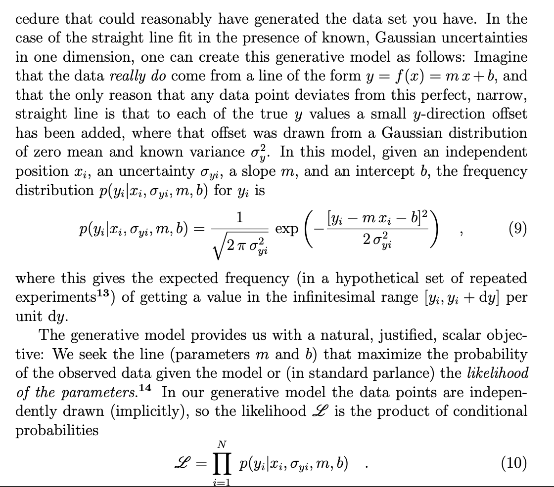
Intro and Chapter 1; pages 1-8
D. Hogg et al. https://arxiv.org/abs/1008.4686
Lots of details about how to properly treat outliers, uncertainties, assumptions in fitting a line to data. Witty comments make it entertaining. Exercise it make it very helpful
D. Hogg et al. https://arxiv.org/abs/1008.4686 - lots of details about how to properly treat outliers, uncertainties, assumptions in fitting a line to data. Witty comments make it entertaining. Exercise it make it very helpful
AstroML Chapter 10 - Intro
HOMLwSKLKerasTF Chapter 4 pages 111-117
Elements of Statistical Learning Chapter 3 Section 1 and 2
uncertainties in measurements
systematic uncertainties
stochastic or random errors
unpredictable uncertainty in a measurement
due to lack of sensitivity in the measurement or
to stochasticity in a process
stochastic or random errors
unpredictable uncertainty in a measurement
due to lack of sensitivity in the measurement or
to stochasticity in a process
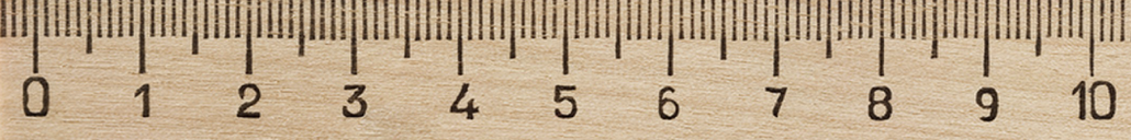
2.5 +/- 0.1 cm
stochastic or random errors
unpredictable uncertainty in a measurement
due to lack of sensitivity in the measurement or
to stochasticity in a process
2.0 +/- ε cm, ε > 0.1 cm
stochastic or random errors
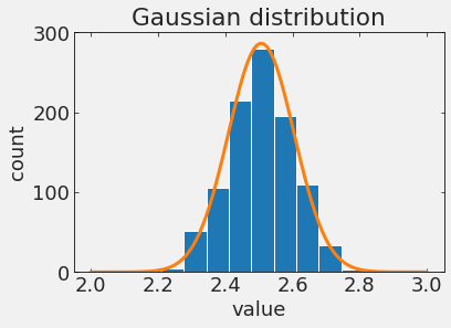
every measurement will be a bit different
2.0 +/- ε cm, ε > 0.1 cm
stochastic or random errors
Deterministic systems have no randomness in
their evolution. Chaos is deterministic.…
Stochastic processes can be
completely random: the probability of any event
is disjoint from that of the previous one
stochastic or random errors
every measurement will be a bit different
2.0 +/- ε cm, ε > 0.1 cm
2.4, 2.6, 2.5, 2.3, 2.4, 2.7, 2.3, 2.5, 2.6, 2.4
stochastic or random errors
2.0 +/- ε cm, ε > 0.1 cm
stochastic or random errors
stochastic or random errors
stochastic or random errors
stochastic or random errors
stochastic or random errors
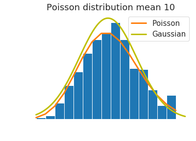
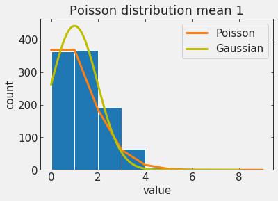
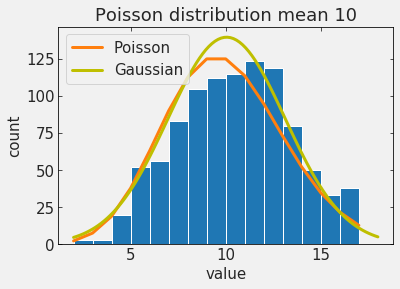
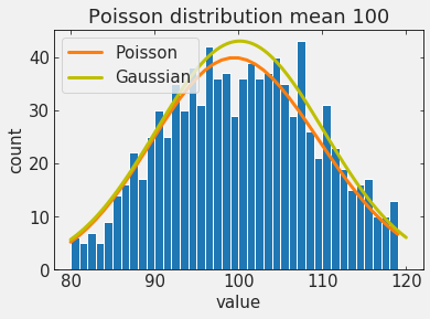
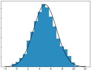
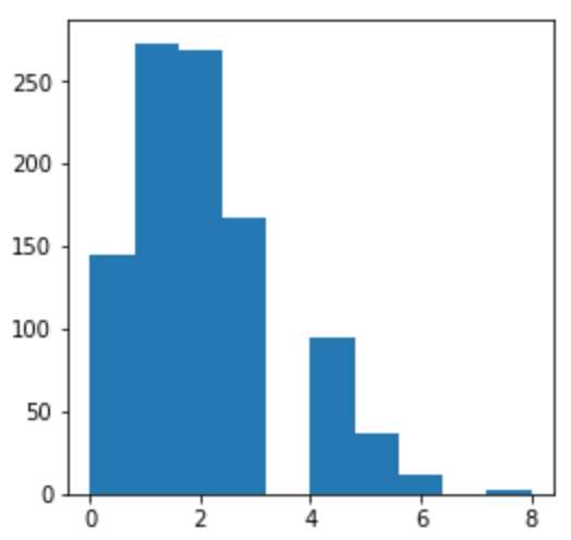
of particular interest are Poisson processes
A discrete distribution that expresses the probability of a number of events
occurring in a fixed period of time if these events occur with a known average rate
and independently of the time since the last event.
stochastic or random errors
of particular interest are Poisson processes
stochastic or random errors
of particular interest are Poisson processes
stochastic or random errors
of particular interest are Poisson processes
as the mean increases it starts looking like a Gaussian!
systematic uncertainties
systematic errors
reproducible inaccuracy introduced by faulty equipment, calibration, or technique.
systematic errors
2.5
reproducible inaccuracy introduced by faulty equipment, calibration, or technique.
2.7 => 2.5 + 0.2 +/- 0.1
systematic errors
2.5
reproducible inaccuracy introduced by faulty equipment, calibration, or technique.
2.7 => 2.5 + 0.2 +/- 0.1
systematic errors
2.5
reproducible inaccuracy introduced by faulty equipment, calibration, or technique.
2.7 => 2.5 + 0.2 +/- 0.1
systematic errors
2.5
reproducible inaccuracy introduced by faulty equipment, calibration, or technique.
2.7 => 2.5 + ? +/- 0.1
systematic errors
inaccuracy introduced by faulty equipment, calibration, or technique.
systematic errors
inaccuracy introduced by faulty equipment, calibration, or technique.
systematic errors
inaccuracy introduced by faulty equipment, calibration, or technique.
the surveyed segment of the population is lower in a sample than it is in the population. This can happen because the frame used to obtain the sample is incomplete or not representative of the population.
Undercoverage bias
Bias in measurements: know your data
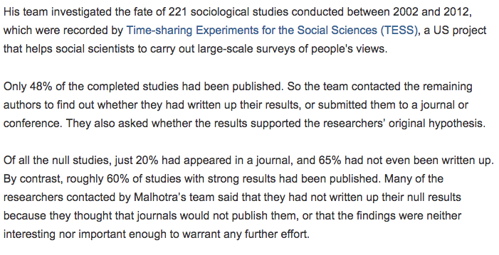
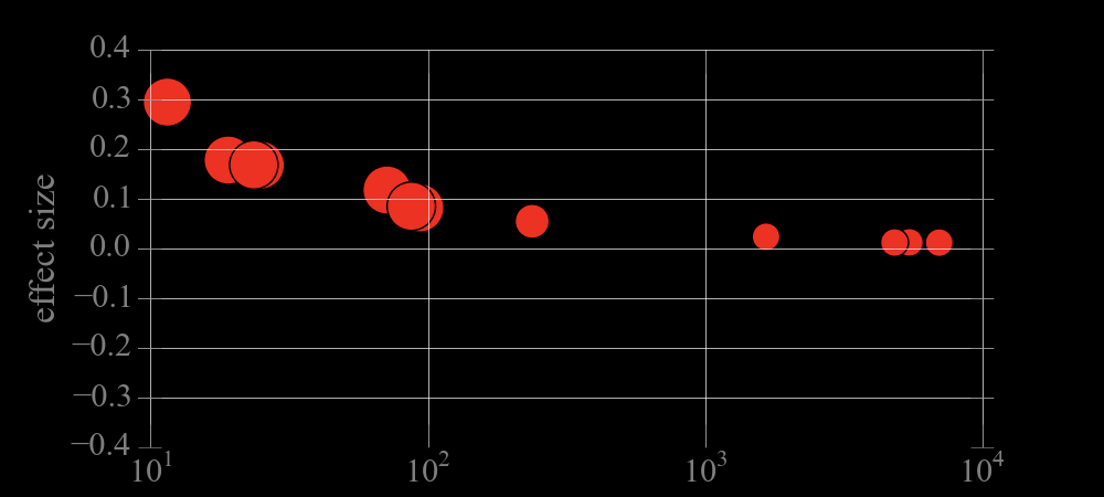
Publication Bias
Bias in measurements: know your data
Publication Bias
Bias in measurements: know your data
Publication Bias
sample size
Bias in measurements: know your data
Publication Bias
sample size
Bias in measurements: know your data
Publication Bias
Bias in measurements: know your data
https://xkcd.com/882/
Data Dredging
Bias in measurements: know your data
Data Dredging
Bias in measurements: know your data
Data Dredging
each test has a
probability p<=0.05
of Type I error
significance 95%
20 tests are preformed
assume independence:
if pi = 0.05 for each i=1..20
Bias in measurements: know your data
Bias in measurements: know your data
Data Dredging
each test has a
probability p<=0.05
of Type I error
significance 95%
20 tests are preformed
assume independence:
if pi = 0.05 for each i=1..20
| Systematic | Statistical |
|---|---|
| Biases the measurement in one direction | No preferred direction |
| Affects the sample regardless of the size | Shrinks with the sample size (typically as N) |
| Any distribution (usually we use Gaussian though) | Typically Gaussian or Poisson |
which relates to stochastic errors,
which to stsystematic?
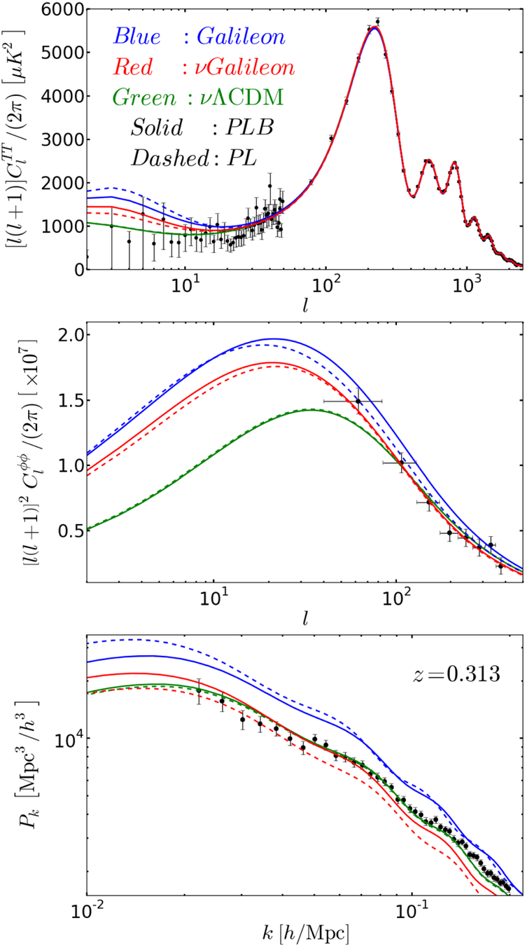
Fig 4: These plots illustrate the differences between 𝛬CDMΛCDM and Galileon models (see Sect. 7.3.1), with and without massive neutrinos. The Galileon models have background Friedmann equations that contain a scalar-field energy density contribution that generates late time cosmic acceleration and has an evolution consistent with observations and thus similar to that of a 𝛬CDMΛCDM model. The Galileon scalar field here also affects linear perturbations and is not coupled to matter. The effect of the Galileon field considered here is focused on large-scale structure. The Top: CMB temperature power spectra showing the ISW effect at low multipoles. Middle: CMB lensing potential spectra. Bottom: linear matter power spectra. The models plotted in dashed lines indicate their best fit models to Ade et al. (2014c) temperature data, WMAP9 polarization data (Hinshaw et al. 2013), and Planck-2013 CMB lensing (Ade et al. 2014d).
They note these as PL models. The solid lines indicate their best fits to CMB data (i.e., PL) plus BAO measurements from 6dF, SDSS DR7 and BOSS DR9. They note these as PLB models. The models correspond to best-fitting base Galileon modified gravity model (in blue), 𝜈GalileonνGalileon (in red) and 𝜈𝛬CDMνΛCDM (in green). For the last two models, the authors added massive neutrino. In the upper and middle panels, the data points show the power spectrum measured by the Planck satellite (Ade et al. 2014c). In the lower panel, the data points show the SDSS-DR7 Luminous Red Galaxy power spectrum of Reid et al. (2010), but scaled down to match the amplitude of the best-fitting 𝜈GalileonνGalileon (PLB) model (Barreira et al. 2014a). We refer to this figure from various parts of the text
Image from Barreira et al. (2014).
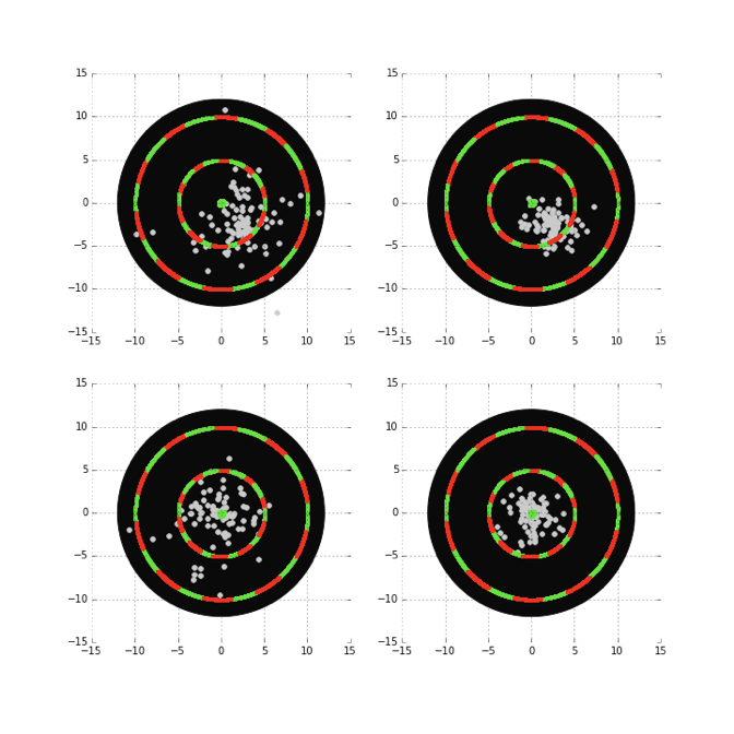
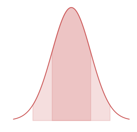
uncertainties: 1-σ
1-σ
68% probability
3 points out of 10 can be outside of the uncertainties
uncertainties: 1-σ
1-σ
68% probability
3 points out of 10 can be outside of the uncertainties
uncertainties: 1-σ
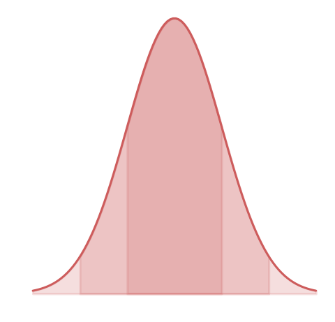
2-σ
95% probability
5 points out of 100 can be outside of the uncertainties
uncertainties: 1-σ
3-σ
99.7% probability
3 points out of 1000 can be outside of the uncertainties
uncertainties: 1-σ
1-σ
68% probability
3 points out of 10 can be outside of the uncertainties
uncertainties: 1-σ
1-σ
68% probability
7 points out of 10 should be inside the errorbar
8 data points:
4 in 4 out
uncertainties: 1-σ
1-σ
68% probability
7 points out of 10 should be inside the errorbar
8 data points:
7 in 1 out
uncertainties: 1-σ
1-σ
68% probability
7 points out of 10 should be inside the errorbar
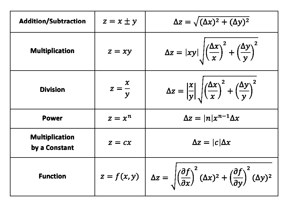
combining uncertainties
If x,…,w are measured with independent and random uncertainties
Δx,…,Δw the uncertainty in a linear combination of x,…,w is the quadratic sum:
If x,y,..,w are measured with independent and random uncertainties
Δx,Δy,…,Δw the uncertainty in a linear combination of x,y,…,w is the quadratic sum:
derivation
derivation
derivation
derivation
sum in quadrature:
derivation
Optimization and Likelihood
6
change a, b to minimize χ2
Target Funcion
Linear regression
Target Funcion
Univariate Linear regression
b
a
Gaussian
Probability of data given a model, e.g. Gaussian
Maximizing the likelihood we seek the parameters that maximize the probability of the observed data under the chosen model
Likelihood: the probability of the model given the data. Same Gaussian assumptions
unknown variables
unknown variables
Target Funcion
Univariate Linear regression
b
a
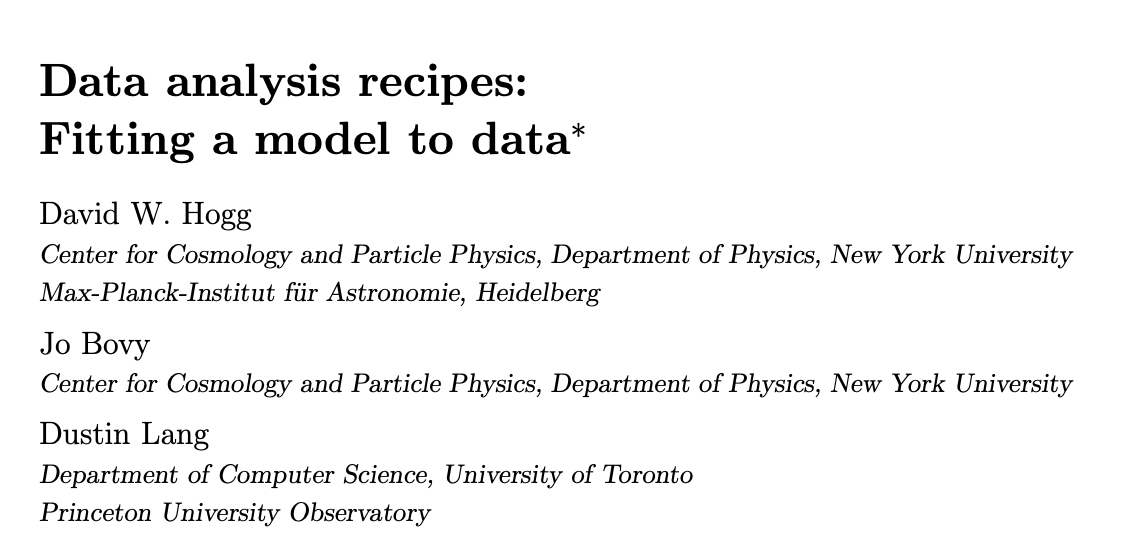
Gradient descent is an iterative algorithm, that starts from a random point on a function and travels down its slope in steps until it reaches the lowest point of that function.
(Toward data science)
Target Funcion
Univariate Linear regression
b
a
Gradient Descent
gradient descent algorithm
"convergence" is reached when the gradient is ~0: with ε tollrance
Target Funcion
Univariate Linear regression
Gradient Descent
Target Funcion
b
a
Target Funcion
b
a
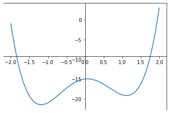
Add stochasticity to avoid getting stuck in a local minimum
stochastic gradient descent algorithm
"convergence" is reached when the gradient is ~0: with ε tollrance
stochastic gradient descent algorithm
"convergence" is reached when the gradient is ~0: with ε tollrance
stochastic gradient descent algorithm
gradient descent algorithm
Target Funcion
Univariate Linear regression
Stochastic Gradient Descent
where i 1 elements of the full N-dimensional observation set (a subset)
Target Funcion
Univariate Linear regression
b
a
idea 2. start a bunch of parallel optimizations
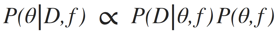
posterior: joint probability distributin of a parameter set (θ, e.g. (m, b)) condition upon some data D and a model hypothesys f
evidence: marginal likelihood of data under the model
prior: “intellectual” knowledge about the model parameters condition on a model hypothesys f. This should come from domain knowledge or knowledge of data that is not the dataset under examination
in reality all of these quantities are conditioned on the shape of the model: this is a model fitting, not a model selection methodology
MonteCarlo methods
results are computed based on repeated random sampling and statistical analysis
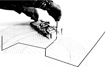
MC history
The number of different games is 52! = 52x51x52…x3x2x1 ~ 8x1067
“What are the chances that a Canfield solitaire laid out with 52 cards will come out successfully?
The number of different games is 52! = 52x51x52…x3x2x1 ~ 8x1067
“What are the chances that a Canfield solitaire laid out with 52 cards will come out successfully?
After spending a lot of time trying to estimate them by pure combinatorial calculations, I wondered whether a more practical method than abstract thinking might not be to lay it out say one hundred times and
simply observe and count the number of successful play”
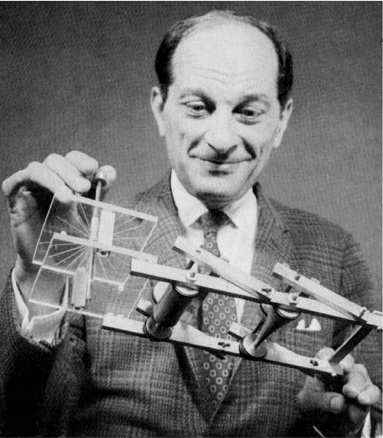
The Fermiac
Enrico Fermi looked really smart with his predictions…
or Monte Carlo trolley
“What are the chances that a Canfield solitaire laid out with 52 cards will come out successfully?
After spending a lot of time trying to estimate them by pure combinatorial calculations, I wondered whether a more practical method than abstract thinking might not be to lay it out say one hundred times and
simply observe and count the number of successful play”
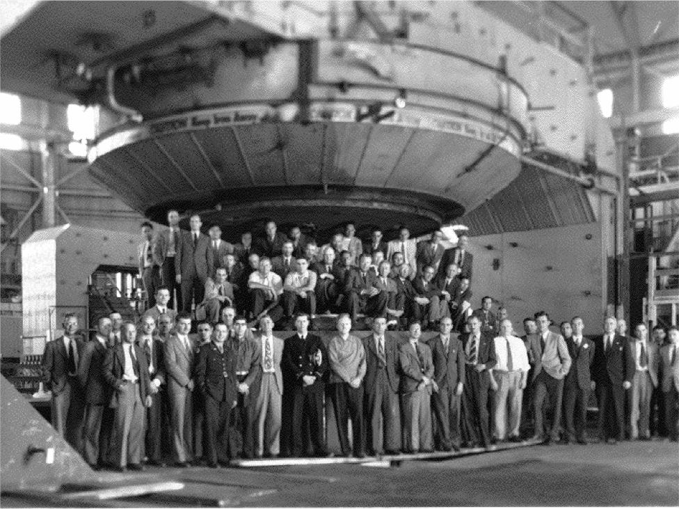
The Manhattan Project
The advent of computing allowed for major innovation in the realm of simulation. Metropolis led a group that developed the Monte Carlo method, which simulates the results of an experiment by using a broad set of random numbers
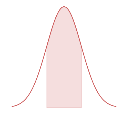
Why am I bothering with areas? - Expectation values are related to areas
Why am I bothering with areas? - Expectation values are related to areas
P(A)
P(C)
P(B)
Why am I bothering with areas? - Expectation values are related to areas
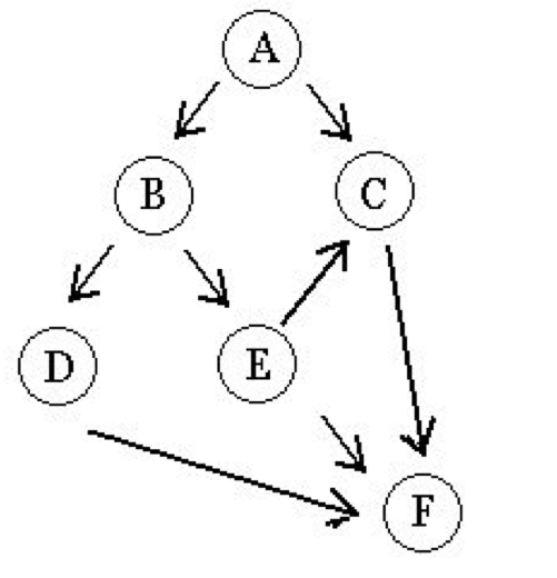
The final probability is likely very complicated (especially if this is a complex system with feedback loops as many physics systems, e.g. radiative transfer!). It may not be tractable analytically but can be simulated
P(F|C,D,E)
Why am I bothering with areas? - Expectation values are related to areas
A person’s depth
B prob to find them at time t
C they survive the avalange
E can be resuscitated at time t
D they are still alive at t
F person survives
Why am I bothering with areas? - Expectation values are related to areas
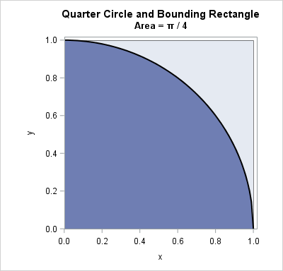
Calculate Pi
https://www.jstor.org/stable/2686489?seq=1
Model Optimization
with MCMC
7
stochastic
"markovian"
sequence
posterior: joint probability distributin of a parameter set (m, b) conditioned upon some data D and a model hypothesys f
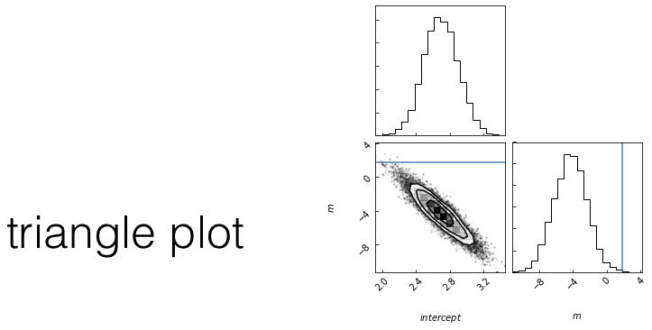
Goal: sample the posterior distribution
slope
intercept
slope
Goal: sample the posterior distribution
choose a starting point in the parameter space: current = θ0 = (m0,b0)
WHILE convergence criterion is met:
calculate the current posterior pcurr = P(D|θ0,f)
//proposal
choose a new set of parameters new = θnew = (mnew,bnew)
calculate the proposed posterior pnew = P(D|θnew,f)
IF pnew/pcurr > 1:
current = new
ELSE:
//probabilistic step: accept with probability pnew/pcurr
draw a random number r ૯U[0,1]
IF pnew/pcurr > r:
current = new
ELSE:
pass // do nothing
stochasticity allows us to explore the whole surface but spend more time in interesting spots
Goal: sample the posterior distribution
choose a starting point in the parameter space: current = θ0 = (m0,b0)
WHILE convergence criterion is met:
calculate the current posterior pcurr = P(D|θ0,f)
//proposal
choose a new set of parameters new = θnew = (mnew,bnew)
calculate the proposed posterior pnew = P(D|θnew,f)
IF pnew/pcurr > 1:
current = new
ELSE:
Questions:
1. how do I choose the next point?
Any Markovian ergodic process
choose a starting point in the parameter space: current = θ0 = (m0,b0)
WHILE convergence criterion is met:
calculate the current posterior pcurr = P(D|θ0,f)
//proposal
choose a new set of parameters new = θnew = (mnew,bnew)
calculate the proposed posterior pnew = P(D|θnew,f)
IF pnew/pcurr > 1:
current = new
ELSE:
//probabilistic step: accept with probability pnew/pcurr
draw a random number r ૯U[0,1]
IF r > pnew/pcurr >:
current = new
ELSE:
pass // do nothing
choose a starting point in the parameter space: current = θ0 = (m0,b0)
WHILE convergence criterion is met:
calculate the current posterior pcurr = P(D|θ0,f)
//proposal
choose a new set of parameters new = θnew = (mnew,bnew)
calculate the proposed posterior pnew = P(D|θnew,f)
IF pnew/pcurr > 1:
current = new
ELSE:
//probabilistic step: accept with probability pnew/pcurr
draw a random number r ૯U[0,1]
IF pnew/pcurr > r:
current = new
ELSE:
pass // do nothing
A process is Markovian if the next state of the system is determined stochastically as a perturbation of the current state of the system, and only the current state of the system, i.e. the system has no memory of earlier states (a memory-less process).
(given enough time) the entire parameter space would be sampled.
At equilibrium, each elementary process should be equilibrated by its reverse process.
reversible Markov process
Detailed Balance is a sufficient condition for ergodicity
Metropolis Rosenbluth Rosenbluth Teller 1953 - Hastings 1970
If the chains are a Markovian Ergodic process
the algorithm is guaranteed to explore the entire likelihood surface given infinite time
This is in contrast to gradient descent, which can get stuck in local minima or in local saddle points.
The problem of fitting models to data reduces to finding the
maximum likelihood
of the data given the model
This is effectively done by finding the minimum of the
-log(likelihood)
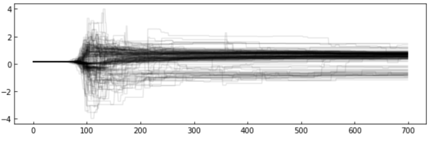
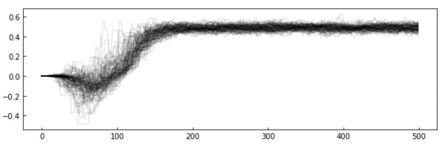
The chains: the algorithm creates a "chain" (a random walk) that "explores" the likelihood surface.
More efficient is to run many parallel chains - each exploring the surface, an "ensemble"
The path of the chains can be shown along each feature
choose a starting point in the parameter space: current = θ0 = (m0,b0)
WHILE convergence criterion is met:
calculate the current posterior pcurr = P(D|θ0,f)
//proposal
choose a new set of parameters new = θnew = (mnew,bnew)
calculate the proposed posterior pnew = P(D|θnew,f)
IF pnew/pcurr > 1:
current = new
ELSE:
//probabilistic step: accept with probability pnew/pcurr
draw a random number r ૯U[0,1]
IF r > pnew/pcurr >:
current = new
ELSE:
pass // do nothing
step
feature value
choose a starting point in the parameter space: current = θ0 = (m0,b0)
WHILE convergence criterion is met:
calculate the current posterior pcurr = P(D|θ0,f)
//proposal
choose a new set of parameters new = θnew = (mnew,bnew)
calculate the proposed posterior pnew = P(D|θnew,f)
IF pnew/pcurr > 1:
current = new
ELSE:
//probabilistic step: accept with probability pnew/pcurr
draw a random number r ૯U[0,1]
IF pnew/pcurr > r:
current = new
ELSE:
pass // do nothing
how to choose the next point
how you make this decision names the algorithm
simulated annealing (good for multimodal)
parallel tempering (good for multimodal)
differential evolution (good for covariant spaces)
Gibbs sampling (move in along one variable at a time)
choose a starting point in the parameter space: current = θ0 = (m0,b0)
WHILE convergence criterion is met:
calculate the current posterior pcurr = P(D|θ0,f)
//proposal
choose a new set of parameters new = θnew = (mnew,bnew)
calculate the proposed posterior pnew = P(D|θnew,f)
IF pnew/pcurr > 1:
current = new
ELSE:
//probabilistic step: accept with probability pnew/pcurr
draw a random number r ૯U[0,1]
IF r > pnew/pcurr >:
current = new
ELSE:
pass // do nothing
step
feature value
choose a starting point in the parameter space: current = θ0 = (m0,b0)
WHILE convergence criterion is met:
calculate the current posterior pcurr = P(D|θ0,f)
//proposal
choose a new set of parameters new = θnew = (mnew,bnew)
calculate the proposed posterior pnew = P(D|θnew,f)
IF pnew/pcurr > 1:
current = new
ELSE:
//probabilistic step: accept with probability pnew/pcurr
draw a random number r ૯U[0,1]
IF pnew/pcurr > r:
current = new
ELSE:
pass // do nothing
Examples of how to choose the next point
affine invariant : EMCEE package
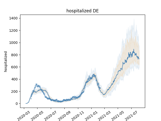
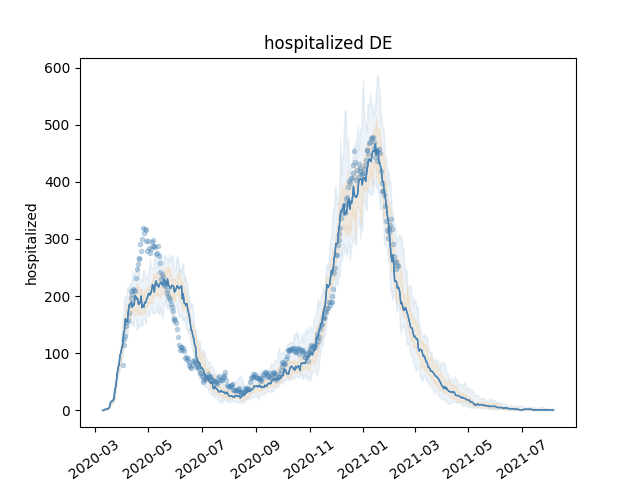
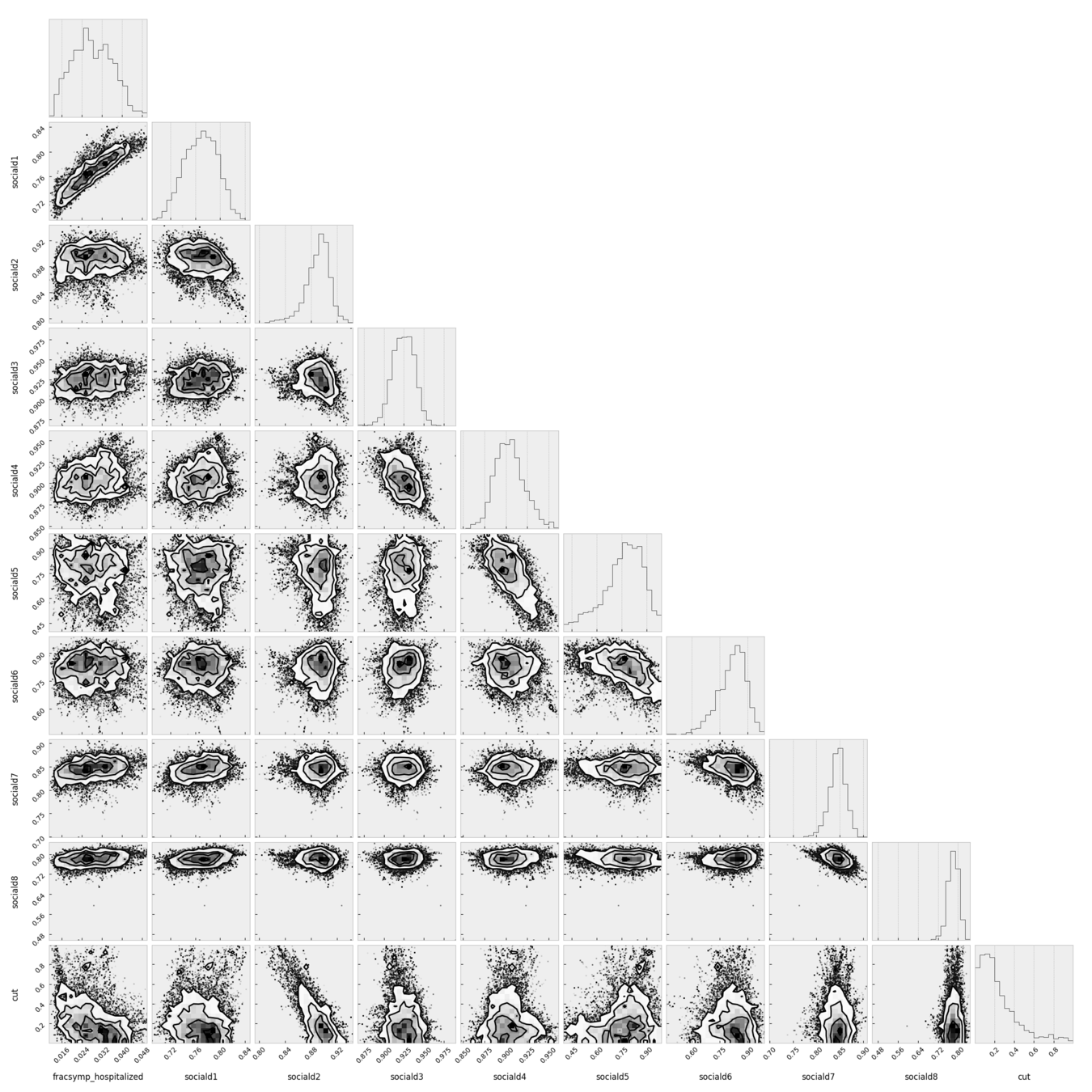
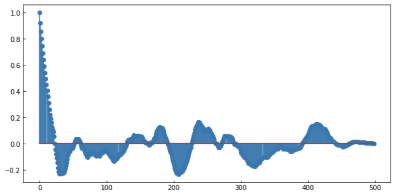
MCMC convergence
MCMC convergence
MCMC convergence
MCMC convergence
MCMC convergence
Principles
8
No matter what anyone tells you an answer to this question cannot be given in the abstract case: it is a domain specific question!
except:
William of Ockham (logician and Franciscan friar) 1300ca
but probably to be attributed to John Duns Scotus (1265–1308)
“Complexity needs not to be postulated without a need for it”
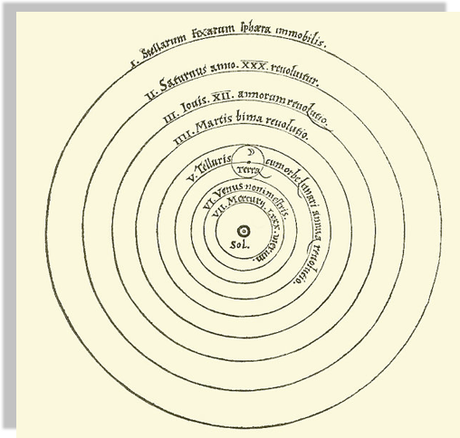
Peter Apian, Cosmographia, Antwerp, 1524 from Edward Grant,
"Celestial Orbs in the Latin Middle Ages", Isis, Vol. 78, No. 2. (Jun., 1987).
Geocentric models are intuitive:
from our perspective we see the Sun moving, while we stay still
the earth is round,
and it orbits around the sun
As observations improve
this model can no longer fit the data!
not easily anyways...
the earth is round,
and it orbits around the sun
Encyclopaedia Brittanica 1st Edition
Dr Long's copy of Cassini, 1777
A new model that is much simpler fit the data just as well
(perhaps though only until better data comes...)
the earth is round,
and it orbits around the sun
Heliocentric model from Nicolaus Copernicus' De revolutionibus orbium coelestium.
William of Ockham (logician and Franciscan friar) 1300ca
but probably to be attributed to John Duns Scotus (1265–1308)
“Complexity needs not to be postulated without a need for it”
“Between 2 theories that perform similarly choose the simpler one”
William of Ockham (logician and Franciscan friar) 1300ca
but probably to be attributed to John Duns Scotus (1265–1308)
“Complexity needs not to be postulated without a need for it”
“Between 2 theories that perform similarly choose the simpler one”
Between 2 theories that perform similarly choose the simpler one
In the context of model selection simpler means "with fewer parameters"
Key Concept
Since all models are wrong the scientist cannot obtain a "correct" one by excessive elaboration. On the contrary following William of Ockham he should seek an economical description of natural phenomena
Since all models are wrong the scientist must be alert to what is importantly wrong.
Science and Statistics George E. P. Box (1976)
Journal of the American Statistical Association, Vol. 71, No. 356, pp. 791-799.
For a dissenting argument
But they should resist it. The value of keeping assumptions to a minimum is cognitive, not ontological: It helps you to think. A theory is not “better” if it is simpler—but it might well be more useful, and that counts for much more.
AIC BIC MLD
8.1
HOW DO I CHOOSE A MODEL?
Given two models which is preferable?
Likelihood-ratio tests
likelihood ratio statistics LR
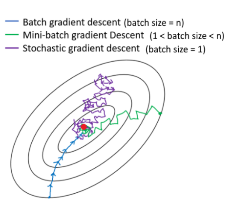
NESTED MODELS : one model contains the other one, e.g.
y= mx + l
is contained in
y=ax**2+ mx + l
statsmodels.model.compare_lr_ratio()
A rigorous answer (in terms of NHST) can be obtained for 2 nested models
This directly answers the question:
“is my more complex model overfitting the data?”
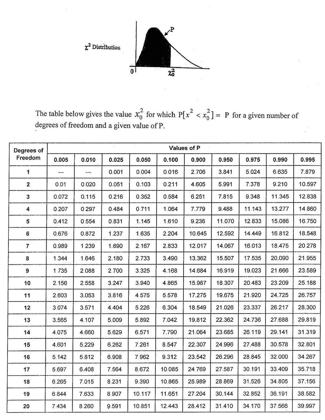
The LR statistics is expected to follow a χ^2 distrbution under the Null Hypothesis that the simpler model is preferable
HOW DO I CHOOSE A MODEL?
Given two models which is preferable?
Likelihood-ratio tests
likelihood ratio statistics LR
statsmodels.model.compare_lr_ratio()
The LR statistics is expected to follow a χ^2 distrbution under the Null Hypothesis that the simpler model is preferable
Shannon 1948: A Mathematical Theory of Communication
a theory to find fundamental limits on signal processing and communication operations such as data compression
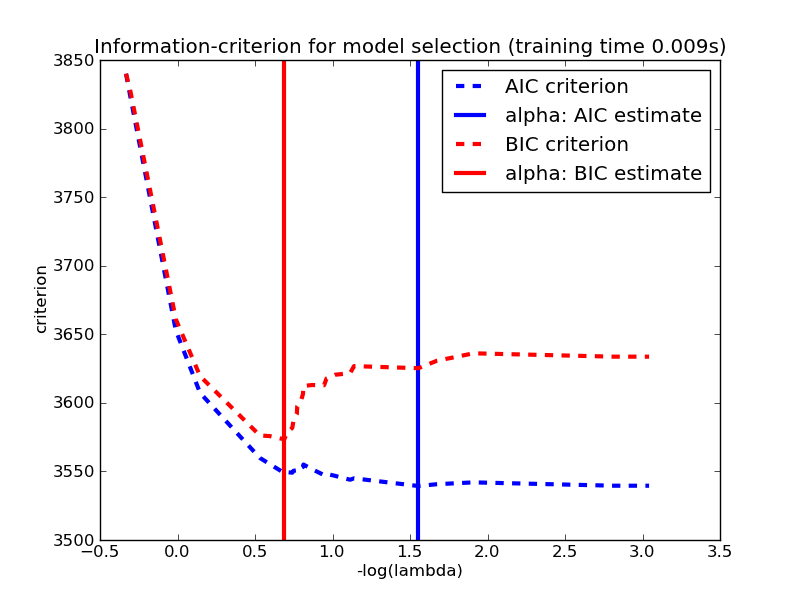
model selection is also based on the minimization of a quantity. Several quantities are suitable:
MLD
BIC
Bayese theorem
AIC
Optimism and likelihood maximization on the training set
Akaike information criterion (AIC) .
Based on
where is a family of function (=densities) containing the correct (=true) function and is the set of parameters that maximized the likelihood L
L is the likelihood of the data, k is the number of parameters,
N the number of variables.
number of parameters:
Model Complexity
Likelihood: Model Performance.
"-" sign in front of the log-likelihood: AIC shrinks for better models,
AIC ~ k => is linearly proportional to the number of parameters
Likelihood: Model Performance.
number of parameters:
Model Complexity
Bayesian information criterion (BIC) .
L is the likelihood of the data, k is the number of parameters,
N the number of variables.
stronger penalization of complexity (as long as N> )
The derivation is very different:
Bayes Factor
Minimum Description Length (MDL) .
negative log-likelihood of the model parameters (θ) and the negative log-likelihood of the target values (y) given the input values (X) and the model parameters (θ).
also: log(L(θ)): number of bits required to represent the model,
log(L(y| X,θ)): number of bits required to represent the predictions on observations
minimize the encoding of the model and its predictions
derived from Shannon's theorem of information
Mathematically similar, though derived from different approaches. All used the same way: the preferred model is the model that minimized the estimator
Elements of Statistical Learning Chapter 7
Sorry ARIMA, but I’m Going Bayesian
https://towardsdatascience.com/implementing-facebook-prophet-efficiently-c241305405a3
read section 1 & 2
By federica bianco
intro to time series and regression


