


federica bianco PRO
astro | data science | data for good
Neural Networks
Fall 2025
dr. federica bianco
@fedhere
this slide deck:
0
Data driven models for exploration of structure, prediction that learn parameters from data.
Data driven models for exploration of structure, prediction that learn parameters from data.
unupervised ------ supervised
set up: All features known for all observations
Goal: explore structure in the data
- data compression
- understanding structure
Algorithms: Clustering, (...)
x
y
Data driven models for exploration of structure, prediction that learn parameters from data.
unupervised ------ supervised
set up: All features known for a sunbset of the data; one feature cannot be observed for the rest of the data
Goal: predicting missing feature
- classification
- regression
Algorithms: regression, SVM, tree methods, k-nearest neighbors, neural networks, (...)
x
y
unupervised ------ supervised
set up: All features known for a sunbset of the data; one feature cannot be observed for the rest of the data
Goal: predicting missing feature
- classification
- regression
Algorithms: regression, SVM, tree methods, k-nearest neighbors, neural networks, (...)
unupervised ------ supervised
set up: All features known for all observations
Goal: explore structure in the data
- data compression
- understanding structure
Algorithms: k-means clustering, agglomerative clustering, density based clustering, (...)
model parameters are learned by calculating a loss function for diferent parameter sets and trying to minimize loss (or a target function and trying to maximize)
e.g.
L1 = |target - prediction|
Learning relies on the definition of a loss function
Learning relies on the definition of a loss function
| learning type | loss / target |
|---|---|
| unsupervised | intra-cluster variance / inter cluster distance |
| supervised | distance between prediction and truth |
The definition of a loss function requires the definition of distance or similarity
Minkowski distance
Jaccard similarity
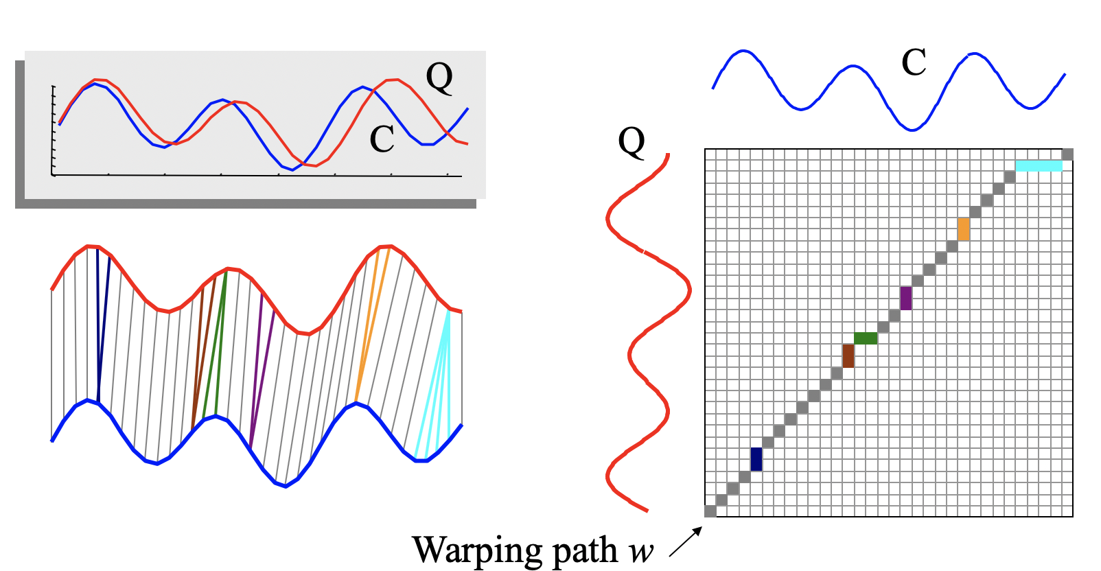
Dynamic Time Warping
The definition of a loss function requires the definition of distance or similarity
The definition of a loss function requires the definition of distance or similarity
Dont confuse the distance definition with the model!!
Models:
Distances:
mikowski
Euclidan
DTW
....
k-mean clusering SVM
kNN
RF
GBT
NN
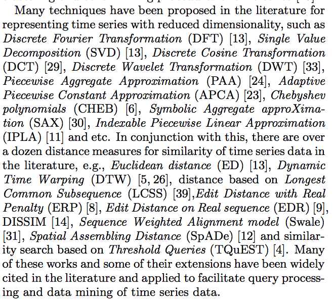
Feature extraction methods == dimensionality reduction:
Dont confuse feature extraction methods with model, tho sometimes models can be used for feature exctraction...
PCA, ICA, clustering, autoencoders...
Finding lower dimensional representation of your data that still preserves similarity and "distance"
In time series he dimensionality is generally the number of data points which is generally very large
Feature extraction methods == dimensionality reduction:
Dont confuse feature extraction methods with model, tho sometimes models can be used for feature exctraction...
Dimensionality reduction:
Distance definitions
Ding et al. 2008
1
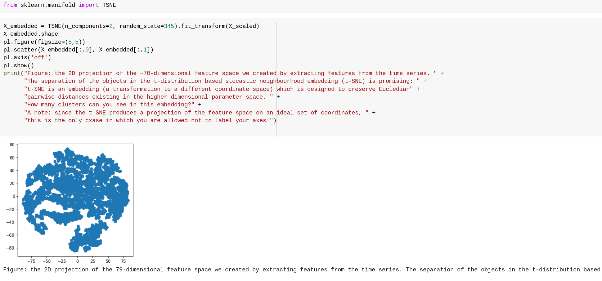
dimensionality reduction techniques are useful both for data preparation (to fight the Curse of Dimensionality) and to enable visualizations of large dataset.
In the latter casewe project a dataset that exists in a high (N)-dimensional space in a lower dimensional (typically 2D) projection with the goal of preserving distances between objects.... but that is really hard!
Proper dimensionality reduction
- LDA ( Linear Discriminant Analysis )
PCA ( Principle Component Analysis )
- ICA ( Independent Component Analysis )
- Clustering (any method, represent data by their cluster)
- Using the latent space of an Autoencoder
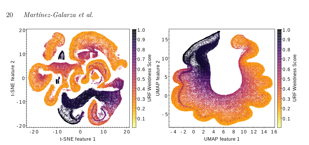
Visualization techniques
- SNE Stochastic Neighborhood Embedding
t-SNE t-distrubuted SNE
- UMAP ( Uniform Manifold Approximation and Projection )
I would say that they are considered primarily visualization techniques, rather than clustering methods or preprocessing tools, because they are very sensitive to the choice of hyperparameter
The t-distributed Stochastic Neighbor Embedding (SNE) method, or t-sne, was introduced in Maaten 2008. SNE works by embedding multidimensional Euclidean distances with conditional probabilities, which is what represents the similarities between datapoints. In other words, suppose we have a data point x_i in the high dimensional space. Then consider a normal distribution of distances from x_i, wherein points near x_i have a higher probability density under the distribution and further points have a lower probability density under the distribution. Then the similarity between x_i and another data point x_i' is the conditional probability P_(x_i' | x_i) that x_i will choose x_i' as a neighbor under the normal distribution just described.
Then we replicate the process for the lower dimensional space, for which we get another set of conditional probabilities. SNE then attempts to minimize the Kullback-Leibler (KL) divergence or relative entropy (Kullback 1951) between the two probability distributions using gradient descent.
Neural Networks
2
NN are a vast topics and we only have 2 weeks!
Some FREE references!
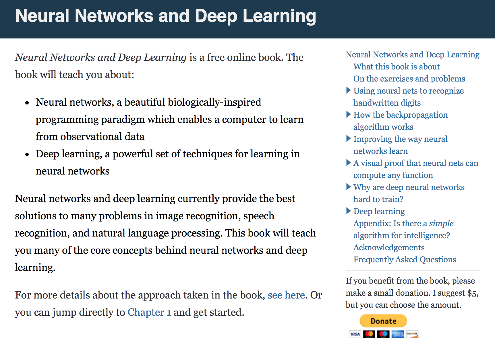
michael nielsen
better pedagogical approach, more basic, more clear
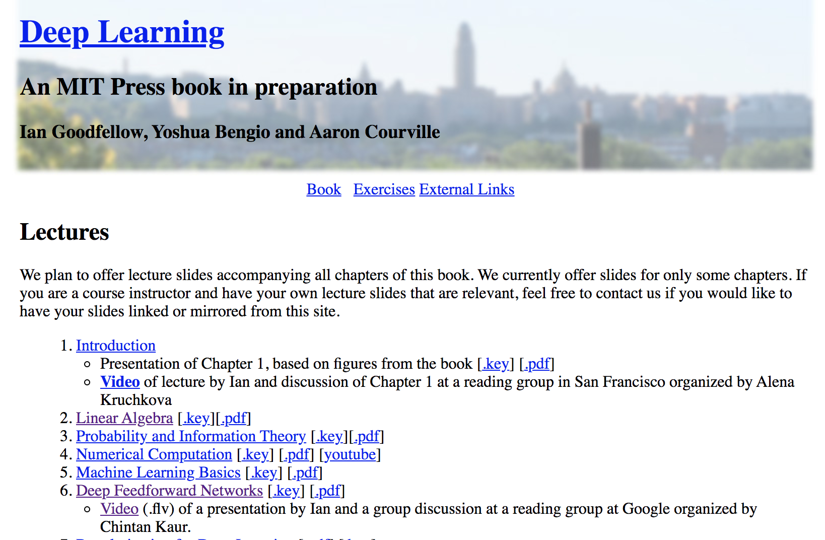
ian goodfellow
mathematical approach, more advanced, unfinished
michael nielsen
better pedagogical approach, more basic, more clear
Neural Networks
2.1
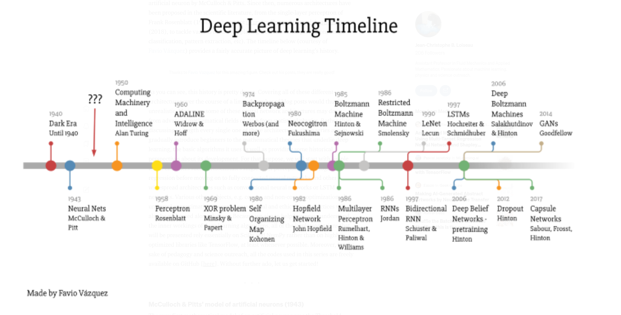
origins
deep
deep
time-domain NN
1943
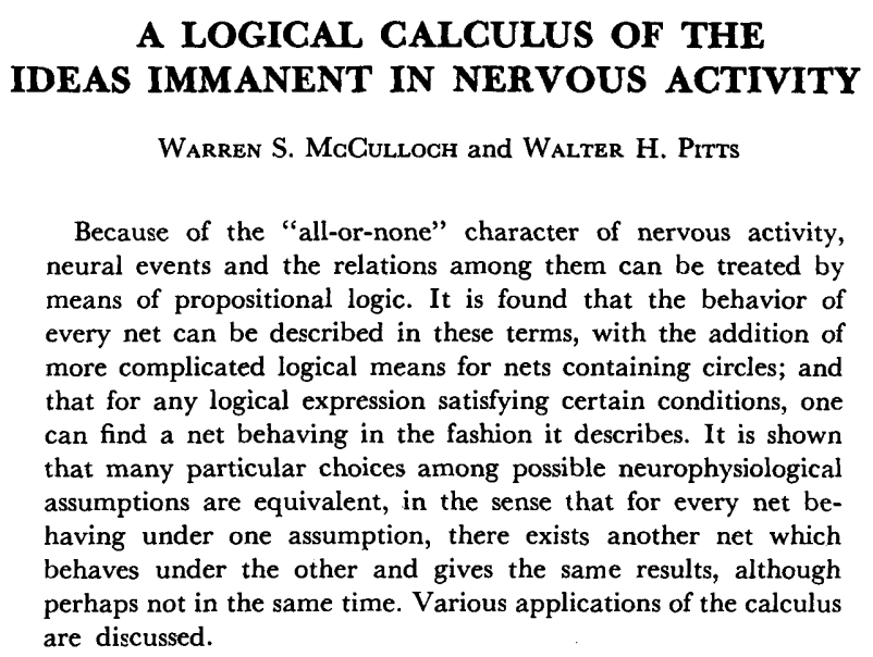
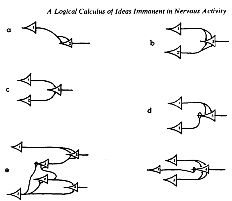
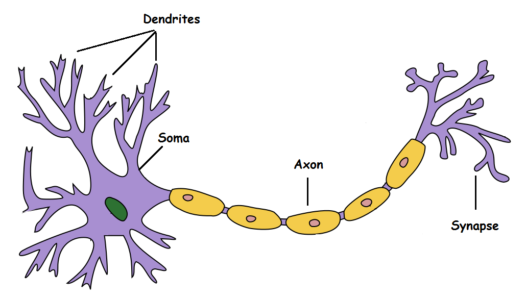
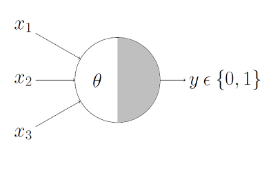
M-P Neuron McCulloch & Pitts 1943
1943
M-P Neuron McCulloch & Pitts 1943
1943
M-P Neuron McCulloch & Pitts 1943
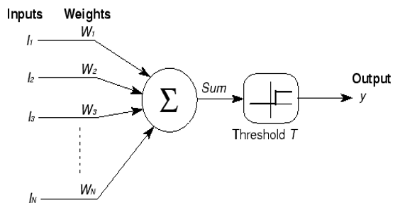
M-P Neuron
1943
M-P Neuron
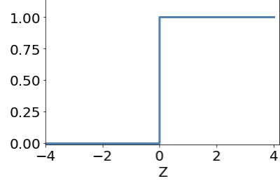
its a classifier
M-P Neuron McCulloch & Pitts 1943
M-P Neuron
1943
M-P Neuron McCulloch & Pitts 1943
M-P Neuron
1943
if
what value of corresponds to logical AND?
M-P Neuron McCulloch & Pitts 1943
Neuron McCulloch & Pitts 1948
1943
.
.
.
output
M-P Neuron
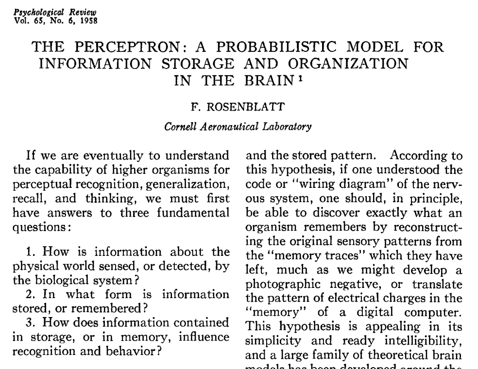
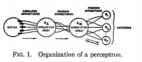
The perceptron algorithm : 1958, Frank Rosenblatt
1958
Perceptron
The perceptron algorithm : 1958, Frank Rosenblatt
.
.
.
output
weights
bias
linear regression:
1958
Perceptron
The perceptron algorithm : 1958, Frank Rosenblatt
.
.
.
output
weights
bias
linear regression:
1958
Perceptron
error
Perceptrons are linear classifiers: makes its predictions based on a linear predictor function
combining a set of weights (=parameters) with the feature vector.
The perceptron algorithm : 1958, Frank Rosenblatt
x
y
1958
output
weights
bias
.
.
.
The perceptron algorithm : 1958, Frank Rosenblatt
Perceptron
The perceptron algorithm : 1958, Frank Rosenblatt
Perceptron
The Navy revealed the embryo of an electronic computer today that it expects will be able to walk, talk, see, write, reproduce itself and be conscious of its existence.
The embryo - the Weather Buerau's $2,000,000 "704" computer - learned to differentiate between left and right after 50 attempts in the Navy demonstration
July 8, 1958
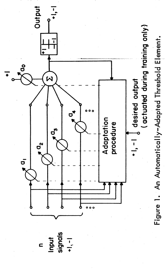
ADALINE : 1960 Bernard Widrow and Ted Hoff
1960
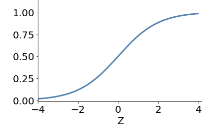
ADALINE introduces a continuous function before the binary output - this generated a probabilistic classifier and provides an opportunity for refining the learning process
.
.
.
output
activation function
weights
bias
error
ADALINE introduces a continuous function before the binary output - this generated a probabilistic classifier and provides an opportunity for refining the learning process
ADALINE : 1960 Bernard Widrow and Ted Hoff
.
.
.
output
activation function
weights
bias
perceptron
ADALINE introduces a continuous function before the binary output - this generated a probabilistic classifier and provides an opportunity for refining the learning process
ADALINE : 1960 Bernard Widrow and Ted Hoff
output
activation function
weights
bias
sigmoid
.
.
.
.
.
.
activation function
ADALINE introduces a continuous function before the binary output - this generated a probabilistic classifier and provides an opportunity for refining the learning process
ADALINE : 1960 Bernard Widrow and Ted Hoff
Weight Change = (Pre-Weight line value)(Error / (Number of Inputs)).
3
1943
AND
OR
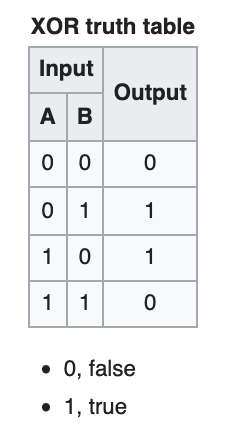
XOR
M-P Neuron McCulloch & Pitts 1943
if x1 and x2 and x3
output
layer of perceptrons
output
input layer
hidden layer
output layer
1970: multilayer perceptron architecture
Fully connected: all nodes go to all nodes of the next layer.
output
layer of perceptrons
output
layer of perceptrons
layer of perceptrons
output
layer of perceptrons
output
Fully connected: all nodes go to all nodes of the next layer.
layer of perceptrons
w: weight
sets the sensitivity of a neuron
b: bias:
up-down weights a neuron
output
Fully connected: all nodes go to all nodes of the next layer.
each perceptron is a multilinear regression
what we are doing is exactly a series of matrix multiplictions.
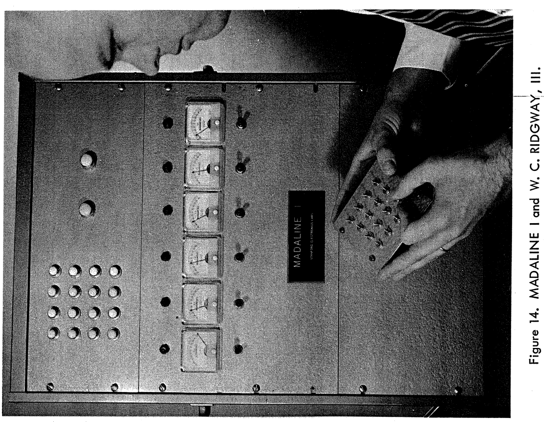
ADELINE and MADELINE 1962 - B. Widrow & M. Hoff
output
Fully connected: all nodes go to all nodes of the next layer.
each perceptron is a multilinear regression
output
Fully connected: all nodes go to all nodes of the next layer.
layer of perceptrons
w: weight
sets the sensitivity of a neuron
b: bias:
up-down weights a neuron
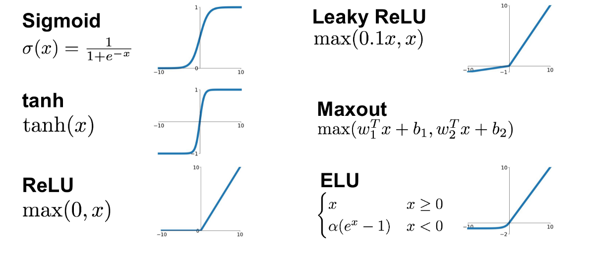
f: activation function:
turns neurons on-off
Fully connected: all nodes go to all nodes of the next layer.
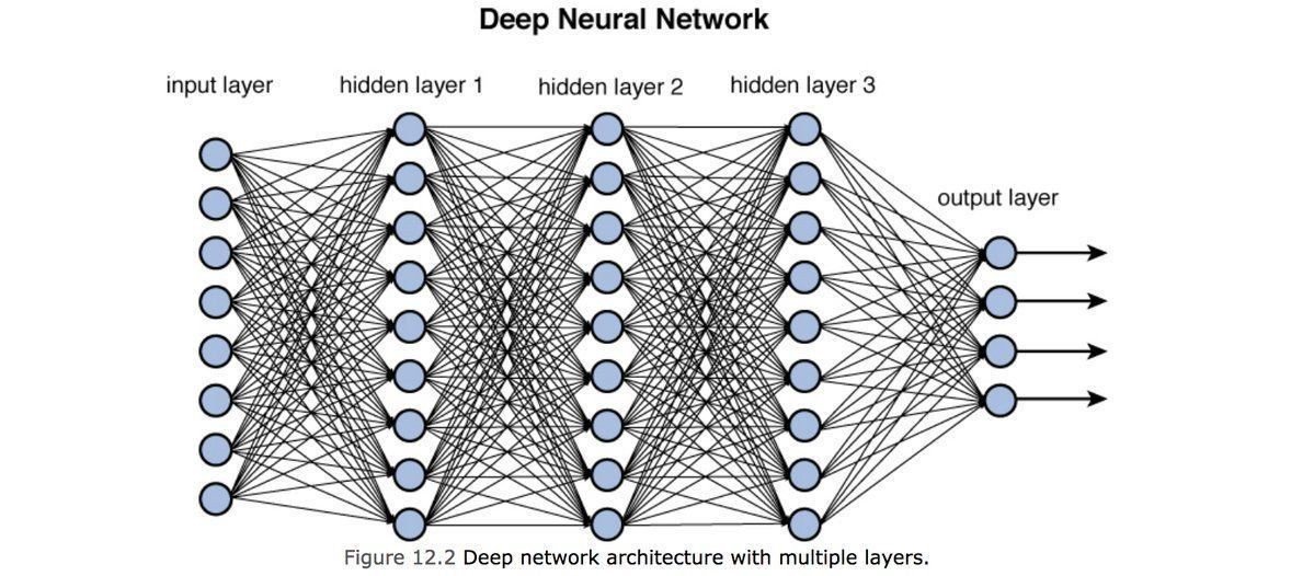
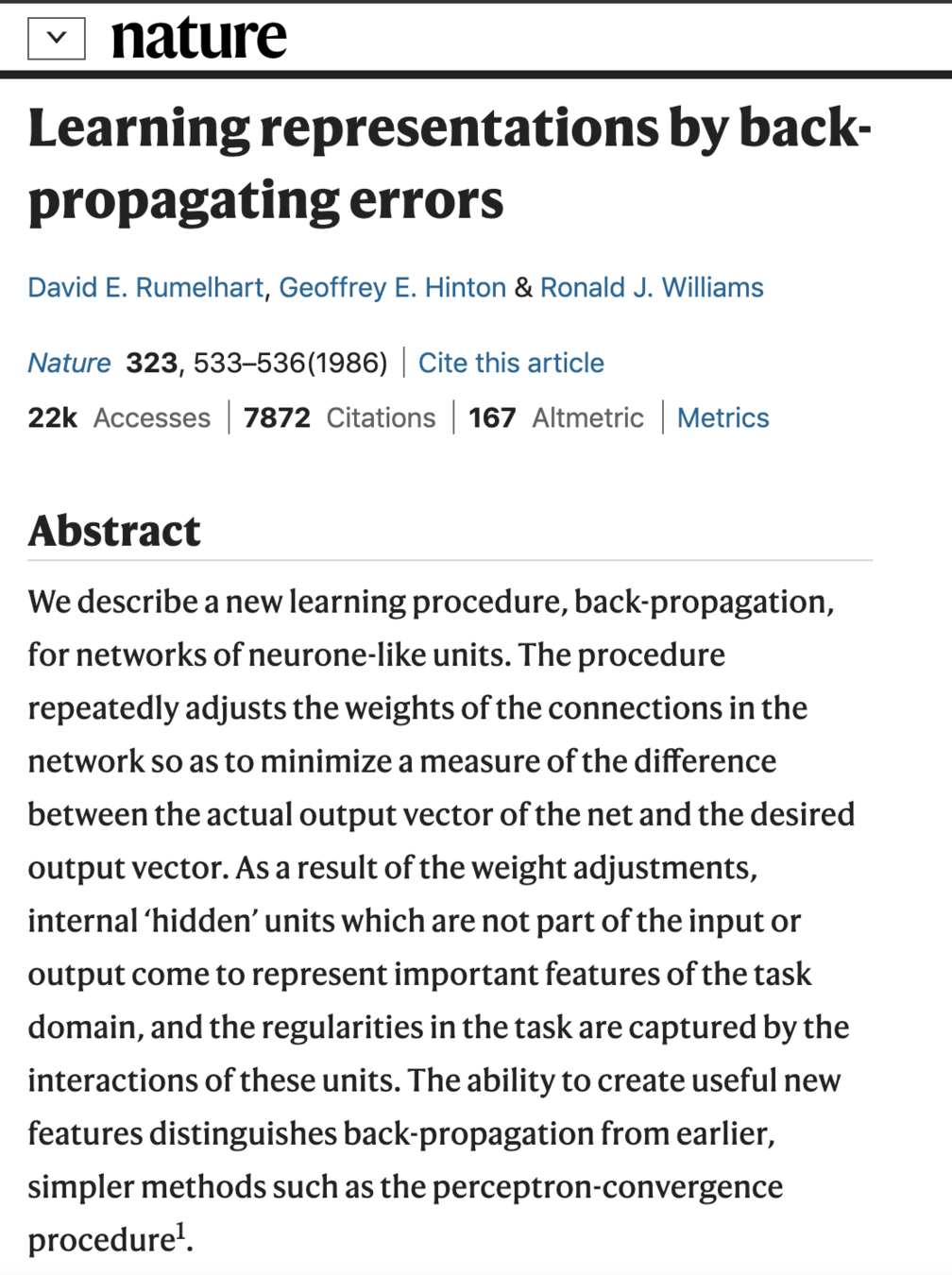
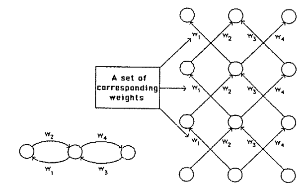
1986: Deep Neural Nets
f: activation function:
turns neurons on-off
w: weight
sets the sensitivity of a neuron
b: bias:
up-down weights a neuron
In a CNN these layers would not be fully connected except the last one
hyperparameters of DNN
4
output
input layer
hidden layer
output layer
hidden layer
how many hyperparameters?
output
input layer
hidden layer
output layer
hidden layer
how many hyperparameters?
Weights
x
Biases
3 x 4 + 4
4 x 3 + 3
3 x 1 + 1
output
input layer
hidden layer
output layer
hidden layer
how many hyperparameters?
Green architecture hyperparameters
RED training parameters
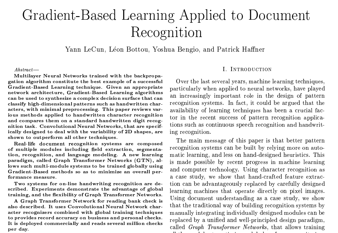
Seminal paper
Y. LeCun 1998
5
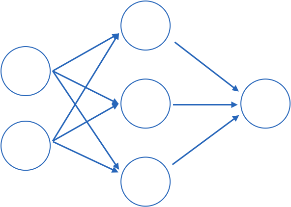
Training models with this many parameters requires a lot of care:
. defining the metric
. optimization schemes
. training/validation/testing sets
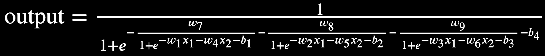
But just like our simple linear regression case, the fact that small changes in the parameters leads to small changes in the output for the right activation functions.
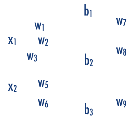
define a cost function, e.g.
x1
x2
b1
b2
b3
b
w11
w12
w13
w21
w22
w23
Lots of parameters and lots of hyperparameters! What to choose?
cheatsheet
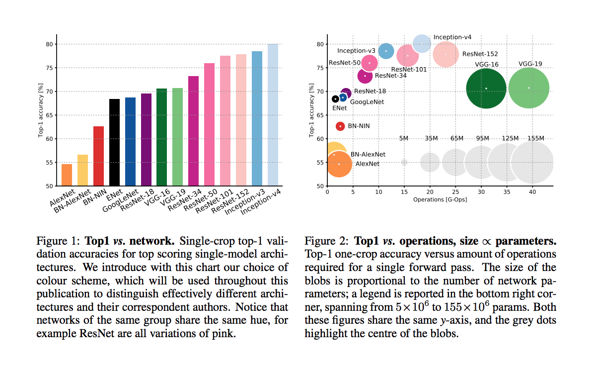
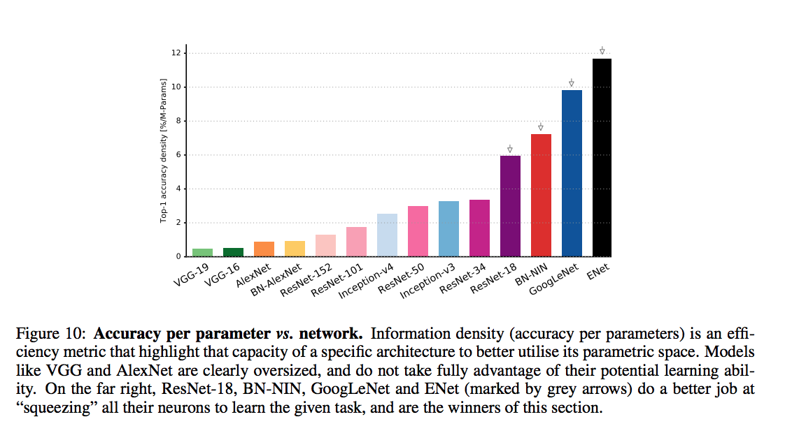
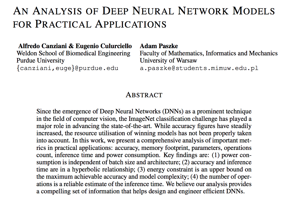
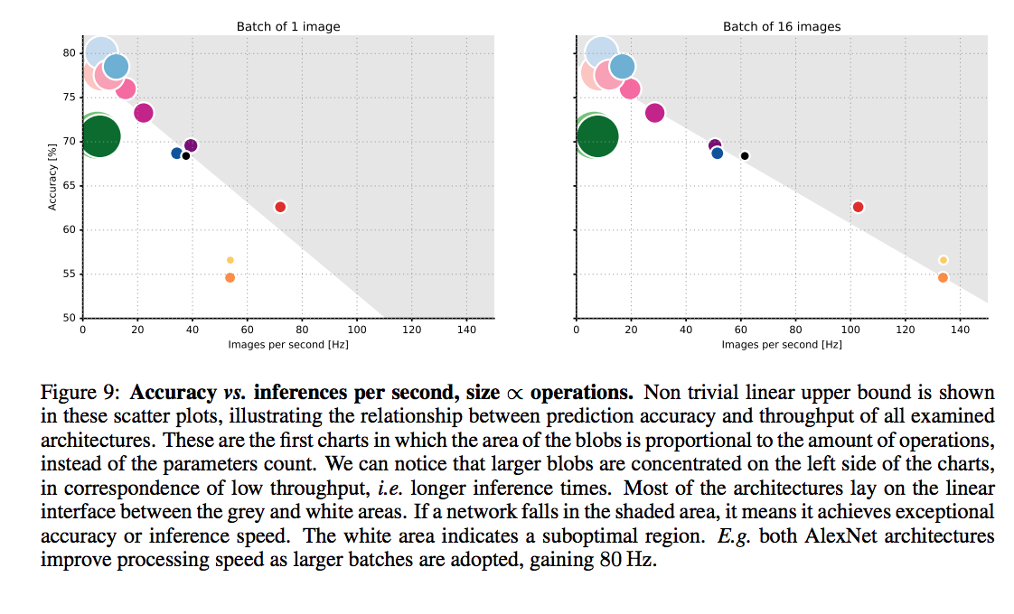
Pretrained DNNs performance comparison
accuracy comparison
An article that compars various DNNs
accuracy comparison
An article that compars various DNNs
batch size
Lots of parameters and lots of hyperparameters! What to choose?
cheatsheet
Lots of parameters and lots of hyperparameters! What to choose?
cheatsheet
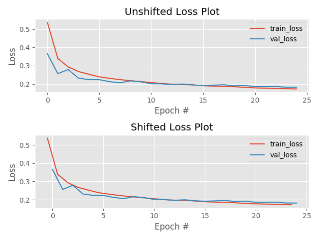
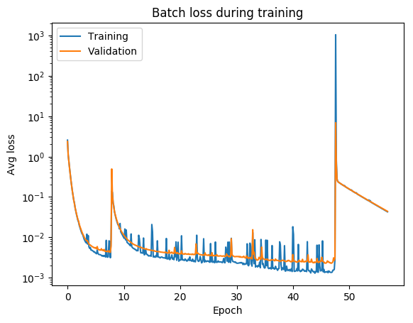
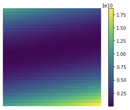
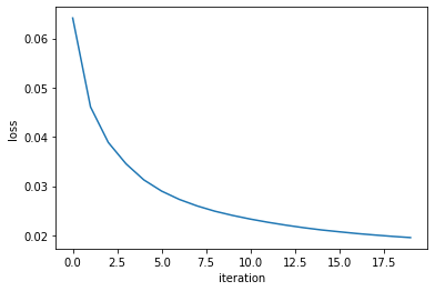
always check your loss function! it should go down smoothly and flatten out at the end of the training.
not flat? you are still learning!
too flat? you are overfitting...
loss (gallery of horrors)
jumps are not unlikely (and not necessarily a problem) if your activations are discontinuous (e.g. relu)
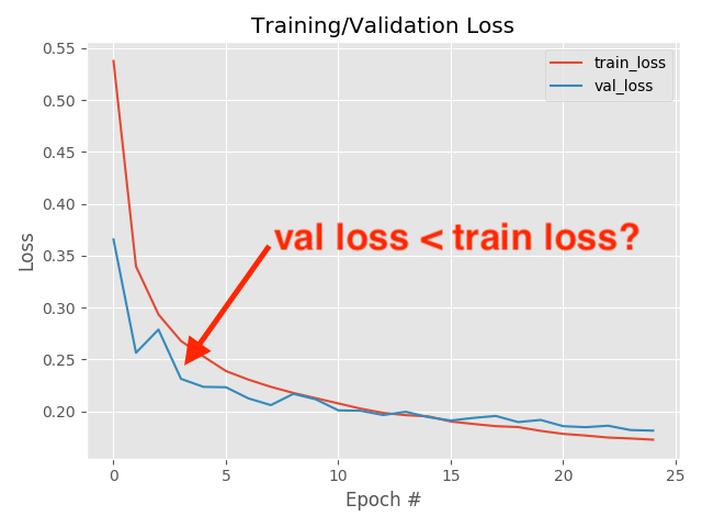
when you use validation you are introducing regularizations (e.g. dropout) so the loss can be smaller than for the training set
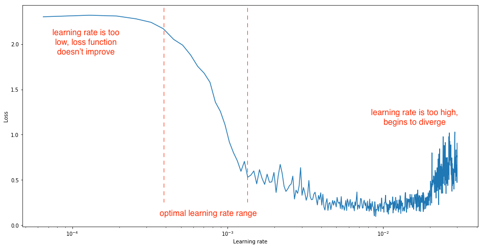
loss and learning rate (not that the appropriate learning rate depends on the chosen optimization scheme!)
Building a DNN
with keras and tensorflow
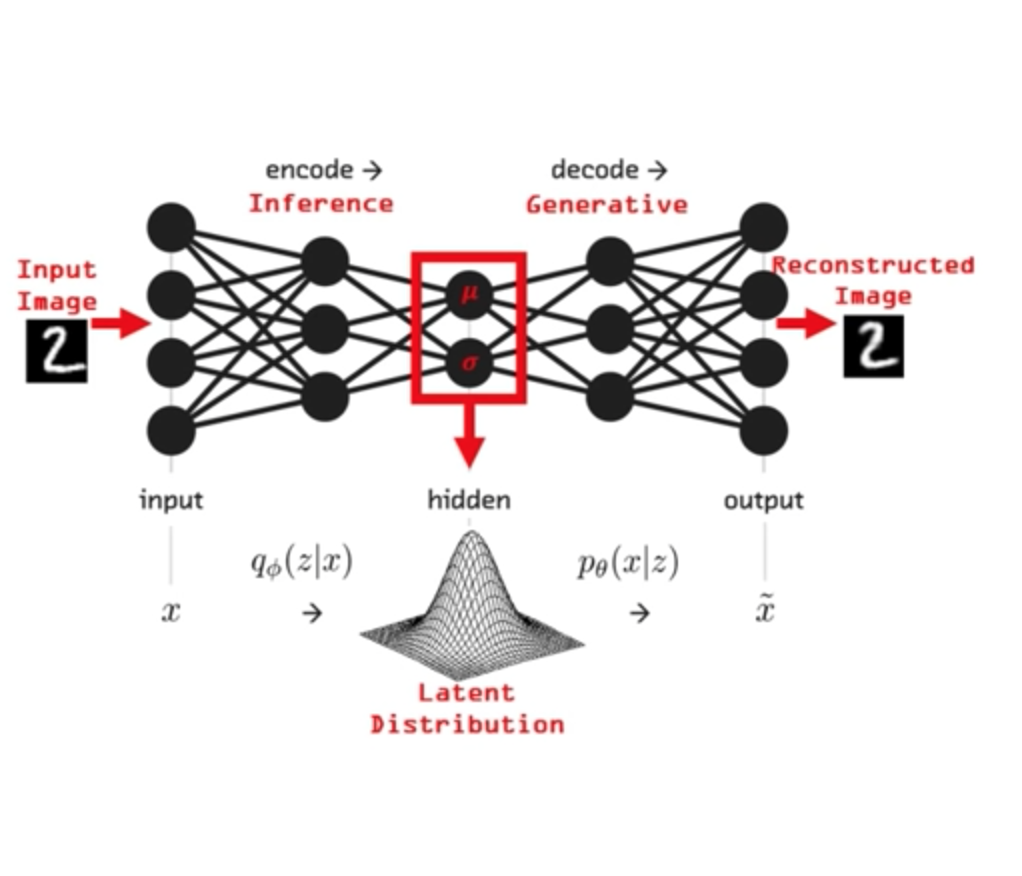
autoencoder for image recontstruction
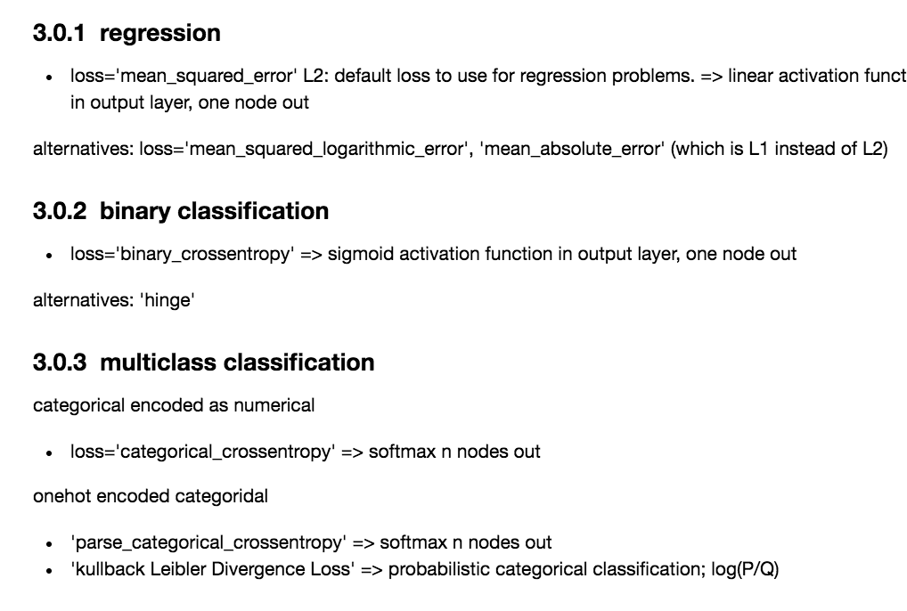
What should I choose for the loss function and how does that relate to the activation functiom and optimization?
| loss | good for | activation last layer | size last layer |
|---|---|---|---|
| mean_squared_error | regression | linear | one node |
| mean_absolute_error | regression | linear | one node |
| mean_squared_logarithmit_error | regression | linear | one node |
| binary_crossentropy | binary classification | sigmoid | one node |
| categorical_crossentropy | multiclass classification | sigmoid | N nodes |
| Kullback_Divergence | multiclass classification, probabilistic inerpretation | sigmoid | N nodes |
Text
Building a DNN
with keras and tensorflow
autoencoder for image recontstruction
| loss | good for | activation last layer | size last layer |
|---|---|---|---|
| mean_squared_error | regression | linear | one node |
| mean_absolute_error | regression | linear | one node |
| mean_squared_logarithmit_error | regression | linear | one node |
| binary_crossentropy | binary classification | sigmoid | one node |
| categorical_crossentropy | multiclass classification | sigmoid | N nodes |
| Kullback_Divergence | multiclass classification, probabilistic inerpretation | sigmoid | N nodes |
in this notebook above I experiment with combinations of these choices
What should I choose for the loss function and how does that relate to the activation functiom and optimization?
Lots of parameters and lots of hyperparameters! What to choose?
training DNN
6
.
.
.
Any linear model:
y : prediction
ytrue : target
Error: e.g.
intercept
slope
L2
x
Find the best parameters by finding the minimum of the L2 hyperplane
at every step look around and choose the best direction
how does linear descent look when you have a whole network structure with hundreds of weights and biases to optimize??
.
.
.
output
Training models with this many parameters requires a lot of care:
. defining the metric
. optimization schemes
. training/validation/testing sets
But just like our simple linear regression case, the fact that small changes in the parameters leads to small changes in the output for the right activation functions.
define a cost function, e.g.
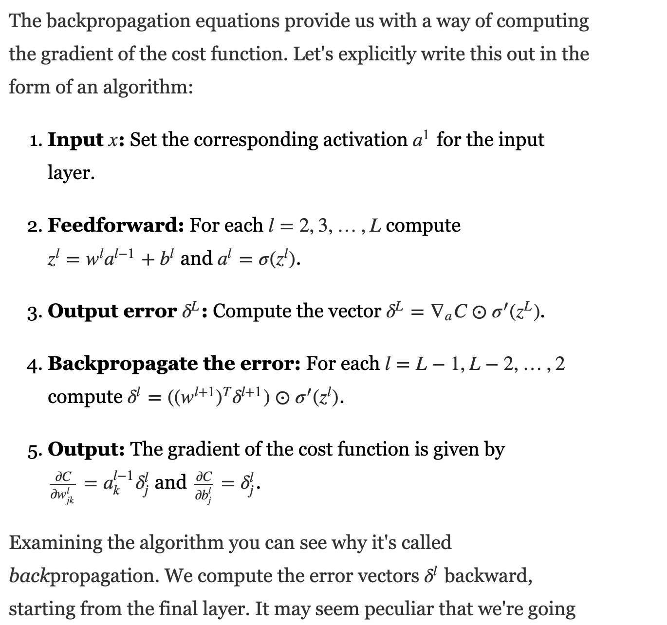
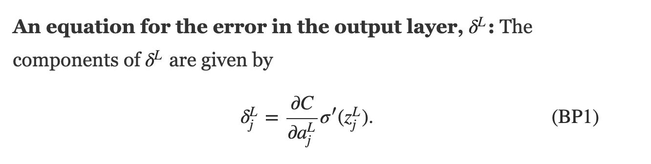
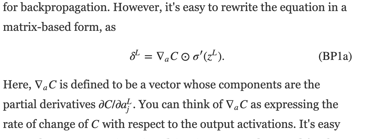
Training a DNN
feed data forward through network and calculate cost metric
for each layer, calculate effect of small changes on next layer
how does linear descent look when you have a whole network structure with hundreds of weights and biases to optimize??
think of applying just gradient to a function of a function of a function... use:
1) partial derivatives, 2) chain rule
define a cost function, e.g.
Training a DNN
Autoencoders
7
Unsupervised learning with
Neural Networks
What do NN do? approximate complex functions with series of linear functions
Unsupervised learning with
Neural Networks
What do NN do? approximate complex functions with series of linear functions
To do that they extract information from the data
Each layer of the DNN produces a representation of the data a "latent representation" .
The dimensionality of that latent representation is determined by the size of the layer (and its connectivity, but we will ignore this bit for now)
.... so if my layers are smaller what I have is a compact representation of the data
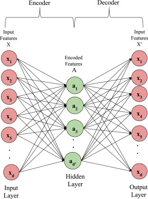
Autoencoder Architecture
Feed Forward DNN:
the size of the input is 5,
the size of the last layer is 2
Autoencoder Architecture
Autoencoder Architecture
Building a DNN
with keras and tensorflow
Trivial to build, but the devil is in the details!
Building a DNN
with keras and tensorflow
Trivial to build, but the devil is in the details!
from keras.models import Sequential
#can upload pretrained models from keras.models
from keras.layers import Dense,  Conv2D, MaxPooling2D
#create model
model = Sequential()


#create the model architecture by adding model layers
model.add(Dense(10, activation='relu', input_shape=(n_cols,)))
model.add(Dense(10, activation='relu'))
model.add(Dense(1))

#need to choose the loss function, metric, optimization scheme
model.compile(optimizer='adam', loss='mean_squared_error')

#need to learn what to look for - always plot the loss function!
model.fit(x_train, y_train, validation_data=(x_test, y_test),
                     epochs=20, batch_size=100, verbose=1)
#note that the model allows to give a validation test,
#this is for a 3fold cross valiation: train-validate-test
#predict
test_y_predictions = model.predict(validate_X)
Building a DNN
with keras and tensorflow
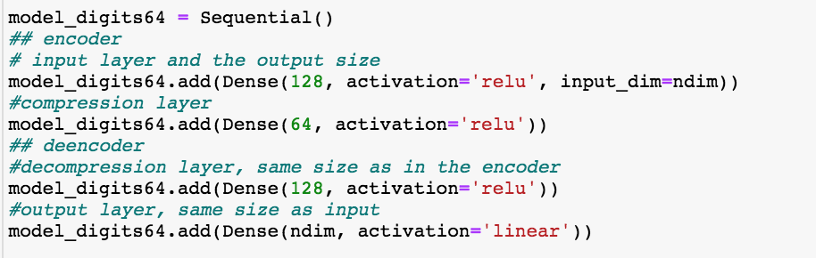
autoencoder for image recontstruction
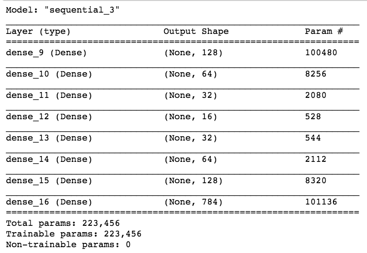
This autoencoder model has a 64-neuron bottle neck. This means it will generate a compressed representation of the data out of that layer which is 16-dimensional (the original size is 784 pixels)
Building a DNN
with keras and tensorflow
autoencoder for image recontstruction
encoder
This autoencoder model has a 64-neuron bottle neck. This means it will generate a compressed representation of the data out of that layer which is 16-dimensional (the original size is 784 pixels)
Building a DNN
with keras and tensorflow
autoencoder for image recontstruction
decoder
This autoencoder model has a 64-neuron bottle neck. This means it will generate a compressed representation of the data out of that layer which is 16-dimensional (the original size is 784 pixels)
Building a DNN
with keras and tensorflow
autoencoder for image recontstruction
This autoencoder model has a 64-neuron bottle neck. This means it will generate a compressed representation of the data out of that layer which is 16-dimensional (the original size is 784 pixels)
bottle neck
Building a DNN
with keras and tensorflow
autoencoder for image recontstruction
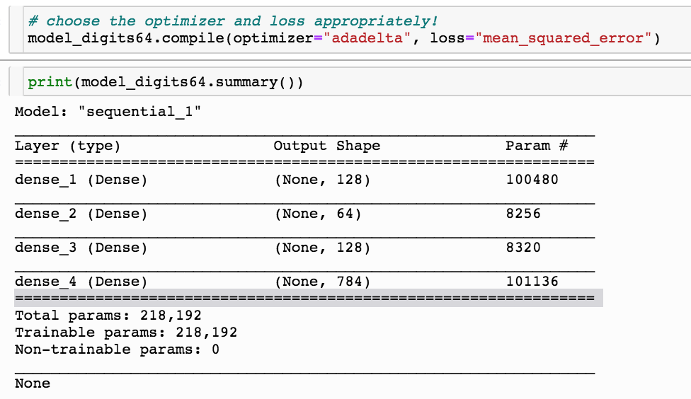
This simple odel has 200000 parameters!
My original choice is to train it with "adadelta" with a mean squared loss function, all activation functions are relu, appropriate for a linear regression
Building a DNN
with keras and tensorflow
autoencoder for image recontstruction
What should I choose for the loss function and how does that relate to the activation functiom and optimization?
Building a DNN
with keras and tensorflow
autoencoder for image recontstruction
What should I choose for the loss function and how does that relate to the activation functiom and optimization?
| loss | good for | activation last layer | size last layer |
|---|---|---|---|
| mean_squared_error | regression | linear | one node |
| mean_absolute_error | regression | linear | one node |
| mean_squared_logarithmit_error | regression | linear | one node |
| binary_crossentropy | binary classification | sigmoid | one node |
| categorical_crossentropy | multiclass classification | sigmoid | N nodes |
| Kullback_Divergence | multiclass classification, probabilistic inerpretation | sigmoid | N nodes |
autoencoder for image recontstruction
model_digits64.add(Dense(ndim,
                        activation='linear'))
model_digits64_sig.compile(optimizer="adadelta",
                   loss="mean_squared_error")
model_digits64_sig.add(Dense(ndim,
activation='sigmoid'))
model_digits64_sig.compile(optimizer="adadelta",
loss="mean_squared_error")
model_digits64_sig.add(Dense(ndim,
activation='sigmoid'))
model_digits64_bce.compile(optimizer="adadelta",
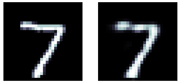
loss="binary_crossentropy")loss function: did not finish learning, it is still decreasing rapidly
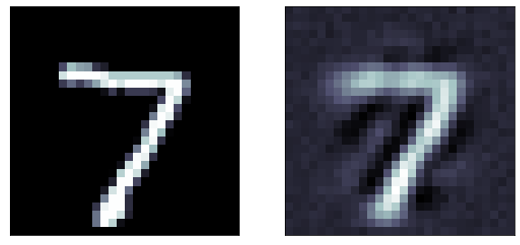
The predictions are far too detailed. While the input is not binary, it does not have a lot of details. Maybe approaching it as a binary problem (with a sigmoid and a binary cross entropy loss) will give better results
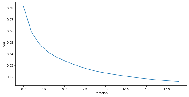
A sigmoid gives activation gives a much better result!
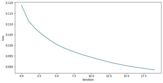
Binary cross entropy loss function: It is more appriopriate when the output layer is sigmoid
Even better results!
original
predicted
predicted
original
predicted
original
predicted
autoencoder for image recontstruction
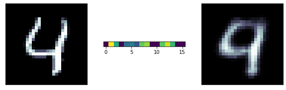
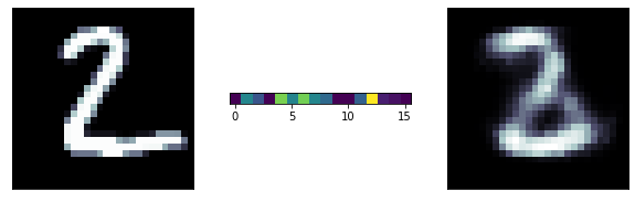
A more ambitious model has a 16 neurons bottle neck: we are trying to extract 16 numbers to reconstruct the entire image! its pretty remarcable! those 16 number are extracted features from the data
predicted
original
latent
representation
Neural Network and Deep Learning
an excellent and free book on NN and DL
http://neuralnetworksanddeeplearning.com/index.html
History of NN
https://cs.stanford.edu/people/eroberts/courses/soco/projects/neural-networks/History/history2.html
Rosenblatt’s perceptron
https://towardsdatascience.com/rosenblatts-perceptron-the-very-first-neural-network-37a3ec09038a
By federica bianco
neural networks


