


federica bianco PRO
astro | data science | data for good
State Space Models and MCMC
Fall 2022 - UDel PHYS 667
dr. federica bianco
@fedhere
combinatorial statistics
Bayes' theorem
optimization
gradient descent
stochastic gradient descent
MCMC
space state models for time series analysis
BSTS fitting
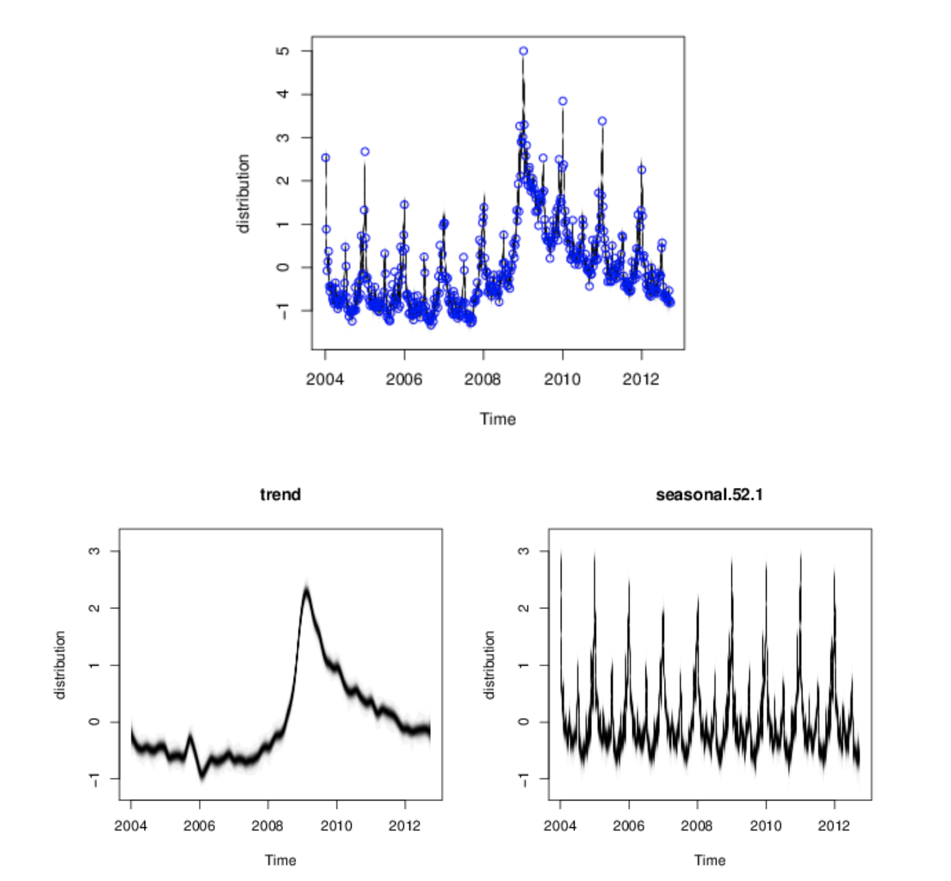
includes descriptions of the local linear trend and seasonal state models, as well as spike and slab priors for regressions with large numbers of predictors.
describes a situation where the local level and local linear trend models would be inappropriate. It offers a semilocal linear trend model as an alternative.
describes a model where the response variable is non-Gaussian. The goal in Example 3 is not to predict the future, but to control for serial dependence in an explanatory model that seeks to identify relevant predictor variables.
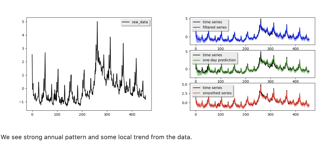
Weekly initial claims for unemployment in the US.
Scott and Varian (2014, 2015)
+
Weekly initial claims for unemployment in the US.
Scott and Varian (2014, 2015)
this slide deck:
Model fit:
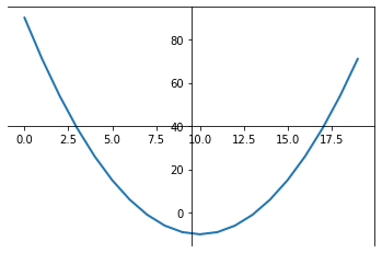
Optimization and Likelihood
1
change a, b to minimize χ2
Target Funcion
Linear regression
Target Funcion
Univariate Linear regression
b
a
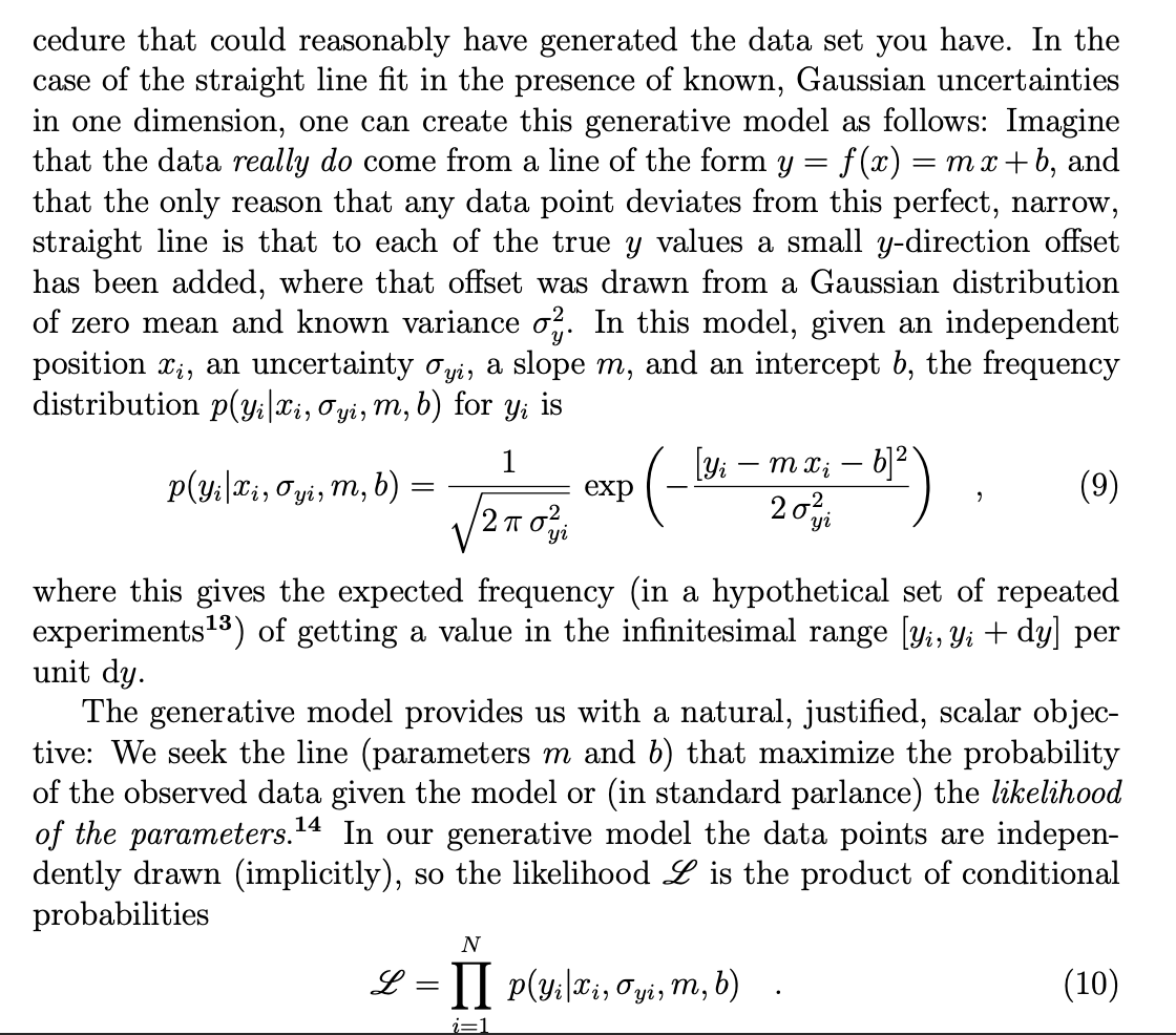
Gaussian
Probability of data given a model, e.g. Gaussian
Maximizing the likelihood we seek the parameters that maximize the probability of the observed data under the chosen model
Likelihood: the probability of the model given the data. Same Gaussian assumptions
unknown variables
unknown variables
Target Funcion
Univariate Linear regression
b
a
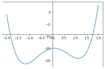
Gradient descent is an iterative algorithm, that starts from a random point on a function and travels down its slope in steps until it reaches the lowest point of that function.
(Toward data science)
Target Funcion
Univariate Linear regression
b
a
Gradient Descent
gradient descent algorithm
"convergence" is reached when the gradient is ~0: with ε tollrance
Target Funcion
Univariate Linear regression
Gradient Descent
Target Funcion
Univariate Linear regression
b
a
Target Funcion
Univariate Linear regression
b
a
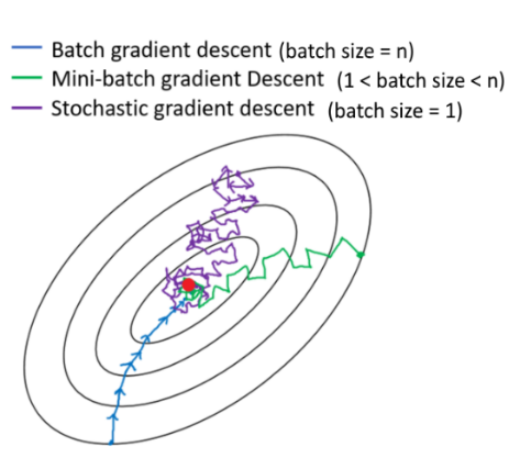
Add stochasticity to avoid getting stuck in a local minimum
stochastic gradient descent algorithm
"convergence" is reached when the gradient is ~0: with ε tollrance
stochastic gradient descent algorithm
"convergence" is reached when the gradient is ~0: with ε tollrance
stochastic gradient descent algorithm
gradient descent algorithm
Target Funcion
Univariate Linear regression
Stochastic Gradient Descent
where i are elements of the full N-dimensional observation set (a subset)
Target Funcion
Univariate Linear regression
b
a
idea 2. start a bunch of parallel optimizations
(we will see it in next class)
Bayes Theorem &
Bayesian statistics
2
probability of A conditioned on B
probability of A conditioned on B
probability of A conditioned on B
probability of A conditioned on B
A and B are independent
probability of A conditioned on B
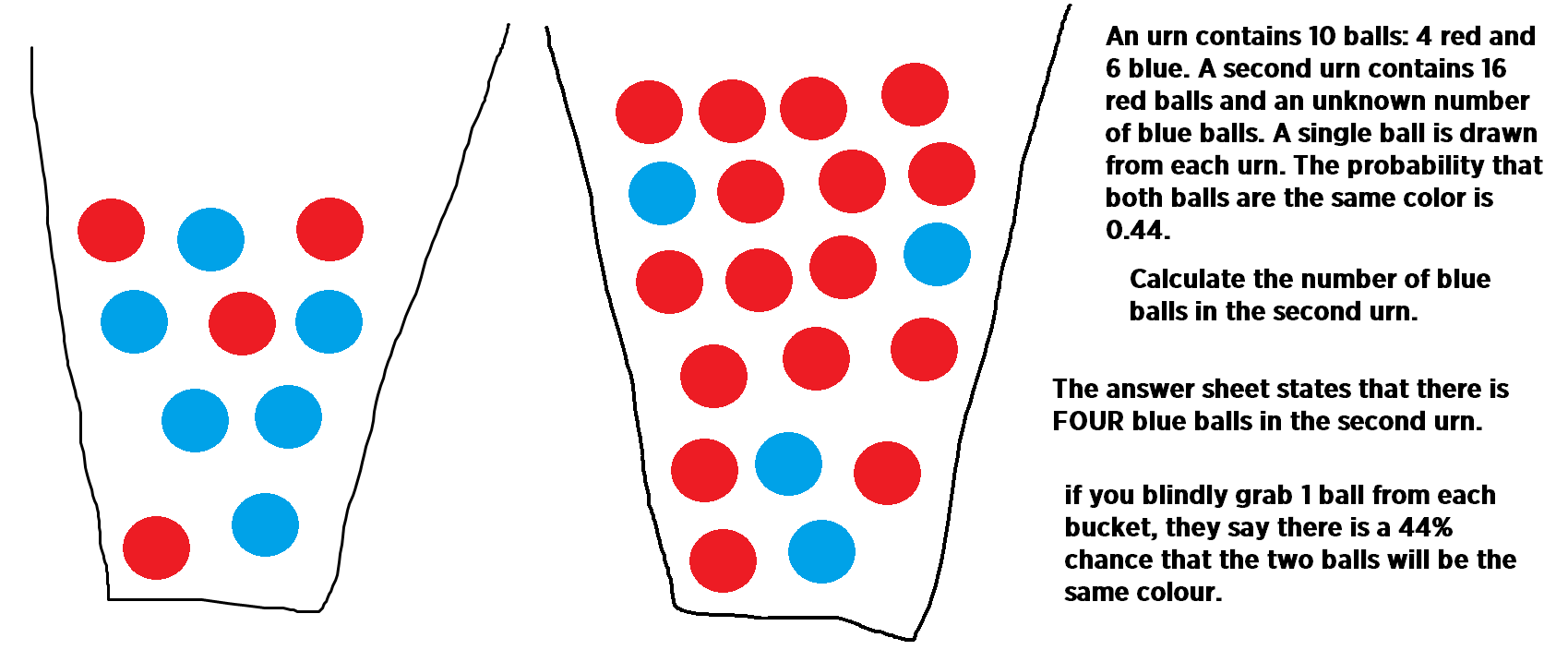
A=red; B=blue
probability of A conditioned on B
A=red; B=blue
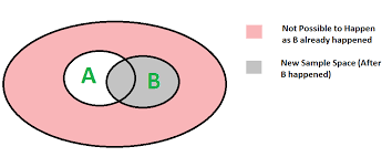
probability of A conditioned on B
new sample space after B happened
A
B
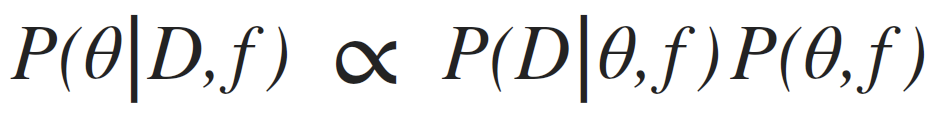
posterior
likelihood
prior
evidence
model parameters
data
D
constraints on the model
e.g. flux from a star is never negative
P(f<0) = 0 P(f>=0) = 1
prior:
model parameters
data
D
model parameters
data
D
prior:
constraints on the model
people's weight <1000lb
& people's weight >0lb
P(w) ~ N(105lb, 90lb)
model parameters
data
D
prior:
constraints on the model
people's weight <1000lb
& people's weight >0lb
P(w) ~ N(105lb, 90lb)
the prior should not be 0 anywhere the probability might exist
model parameters
data
D
prior:
"uninformative prior"
model parameters
data
D
prior:
"uninformative prior"
likelihood:
this is our model
model parameters
data
D
evidence
????
model parameters
data
D
evidence
????
model parameters
data
D
it does not matter if I want to use this for model comparison
model parameters
data
D
it does not matter if I want to use this for model comparison
which has the highest posterior probability?
posterior: joint probability distributin of a parameter set (θ, e.g. (m, b)) condition upon some data D and a model hypothesys f
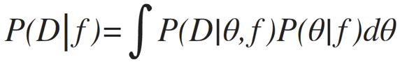
evidence: marginal likelihood of data under the model
prior: “intellectual” knowledge about the model parameters condition on a model hypothesys f. This should come from domain knowledge or knowledge of data that is not the dataset under examination
posterior: joint probability distributin of a parameter set (θ, e.g. (m, b)) condition upon some data D and a model hypothesys f
evidence: marginal likelihood of data under the model
prior: “intellectual” knowledge about the model parameters condition on a model hypothesys f. This should come from domain knowledge or knowledge of data that is not the dataset under examination
in reality all of these quantities are conditioned on the shape of the model: this is a model fitting, not a model selection methodology
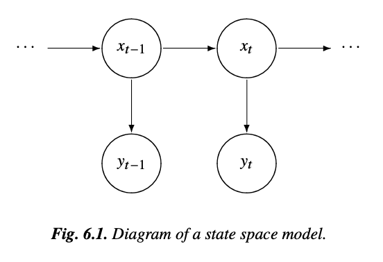
State Space Model
4
motion equations for the position or "state" of a spacecraft
x(t): location
y(t): information that can be observed from a tracking device such as velocity and azimuth
unobserved state
Underlying state x is a time varying Markovian process (the position of the spacecraft)
The observed variable depends at least on the state and on noise.
Other elements (e.g. seasonality) can be included in the model too
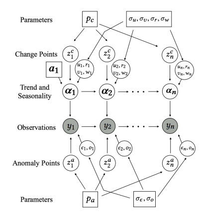
we can write a Bayesian structural model like this:
local level
state
seasonal trend
we can write a Bayesian structural model like this:
seasonal variations
unobserved trend
Its a Markovian Process:
stochastic process with 1-step memory
there is a hidden or latent process xt called the state process (the position of the space craft)
a bit more complex
A model that accepts regression on exogenous variables allows feature extraction: which features are important in the prediction?
e.g. CO2 or Irradiance in climate change (HW)
Model Optimization
with MCMC
5
stochastic
"markovian"
sequence
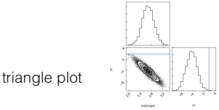
posterior: joint probability distributin of a parameter set (m, b) conditioned upon some data D and a model hypothesys f
Goal: sample the posterior distribution
slope
intercept
slope
Goal: sample the posterior distribution
choose a starting point in the parameter space: current = θ0 = (m0,b0)
WHILE convergence criterion is met:
calculate the current posterior pcurr = P(D|θ0,f)
//proposal
choose a new set of parameters new = θnew = (mnew,bnew)
calculate the proposed posterior pnew = P(D|θnew,f)
IF pnew/pcurr < 1:
current = new
ELSE:
//probabilistic step: accept with probability pnew/pcurr
draw a random number r ૯U[0,1]
IF r > pnew/pcurr >:
current = new
ELSE:
pass // do nothing
stochasticity allows us to explore the whole surface but spend more time in interesting spots
Goal: sample the posterior distribution
choose a starting point in the parameter space: current = θ0 = (m0,b0)
WHILE convergence criterion is met:
calculate the current posterior pcurr = P(D|θ0,f)
//proposal
choose a new set of parameters new = θnew = (mnew,bnew)
calculate the proposed posterior pnew = P(D|θnew,f)
IF pnew/pcurr > 1:
current = new
ELSE:
Questions:
1. how do I choose the next point?
Any Markovian ergodic process
choose a starting point in the parameter space: current = θ0 = (m0,b0)
WHILE convergence criterion is met:
calculate the current posterior pcurr = P(D|θ0,f)
//proposal
choose a new set of parameters new = θnew = (mnew,bnew)
calculate the proposed posterior pnew = P(D|θnew,f)
IF pnew/pcurr > 1:
current = new
ELSE:
//probabilistic step: accept with probability pnew/pcurr
draw a random number r ૯U[0,1]
IF r > pnew/pcurr >:
current = new
ELSE:
pass // do nothing
A process is Markovian if the next state of the system is determined stochastically as a perturbation of the current state of the system, and only the current state of the system, i.e. the system has no memory of earlier states (a memory-less process).
(given enough time) the entire parameter space would be sampled.
At equilibrium, each elementary process should be equilibrated by its reverse process.
reversible Markov process
Detailed Balance is a sufficient condition for ergodicity
Metropolis Rosenbluth Rosenbluth Teller 1953 - Hastings 1970
If the chains are a Markovian Ergodic process
the algorithm is guaranteed to explore the entire likelihood surface given infinite time
This is in contrast to gradient descent, which can get stuck in local minima or in local saddle points.
how to choose the next point
how you make this decision names the algorithm
simulated annealing (good for multimodal)
parallel tempering (good for multimodal)
differential evolution (good for covariant spaces)
Gibbs sampling (move in along one variable at a time)
choose a starting point in the parameter space: current = θ0 = (m0,b0)
WHILE convergence criterion is met:
calculate the current posterior pcurr = P(D|θ0,f)
//proposal
choose a new set of parameters new = θnew = (mnew,bnew)
calculate the proposed posterior pnew = P(D|θnew,f)
IF pnew/pcurr > 1:
current = new
ELSE:
//probabilistic step: accept with probability pnew/pcurr
draw a random number r ૯U[0,1]
IF r > pnew/pcurr >:
current = new
ELSE:
pass // do nothing
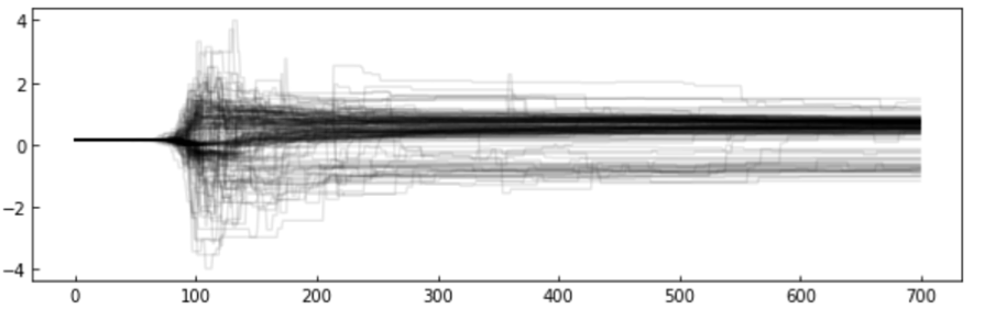
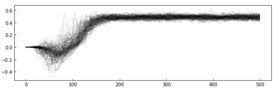
The chains: the algorithm creates a "chain" (a random walk) that "explores" the likelihood surface.
More efficient is to run many parallel chains - each exploring the surface, an "ensemble"
The path of the chains can be shown along each feature
choose a starting point in the parameter space: current = θ0 = (m0,b0)
WHILE convergence criterion is met:
calculate the current posterior pcurr = P(D|θ0,f)
//proposal
choose a new set of parameters new = θnew = (mnew,bnew)
calculate the proposed posterior pnew = P(D|θnew,f)
IF pnew/pcurr > 1:
current = new
ELSE:
//probabilistic step: accept with probability pnew/pcurr
draw a random number r ૯U[0,1]
IF r > pnew/pcurr >:
current = new
ELSE:
pass // do nothing
step
feature value
Examples of how to choose the next point
affine invariant : EMCEE package
choose a starting point in the parameter space: current = θ0 = (m0,b0)
WHILE convergence criterion is met:
calculate the current posterior pcurr = P(D|θ0,f)
//proposal
choose a new set of parameters new = θnew = (mnew,bnew)
calculate the proposed posterior pnew = P(D|θnew,f)
IF pnew/pcurr > 1:
current = new
ELSE:
//probabilistic step: accept with probability pnew/pcurr
draw a random number r ૯U[0,1]
IF r > pnew/pcurr >:
current = new
ELSE:
pass // do nothing
step
feature value
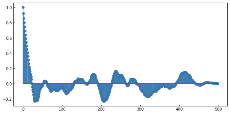
MCMC convergence
MCMC convergence
MCMC convergence
MCMC convergence
MCMC convergence
OF THE WEEK
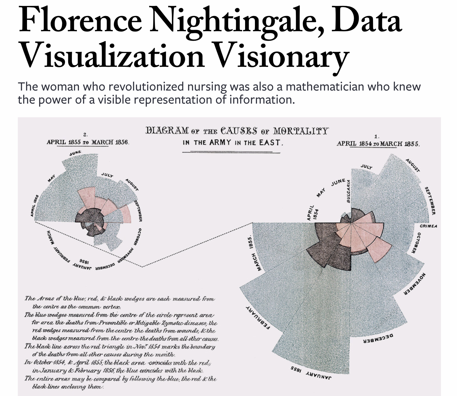
when to do circles?
cyclic visualizations
(annual behavior)
when you do not want to impress importance on the hierarchical time order
Elements of Statistical Learning Chapter 7
https://towardsdatascience.com/implementing-facebook-prophet-efficiently-c241305405a3
By federica bianco
Bayes theorem and MCMC


