What I will present

Theory for minimizing movement schemes in infinite dimensions and in nonsmooth (nondifferentiable) settings, with a movement limiter given by a general cost function.

Main motivation: optimization on a space of measures $\mathcal{P}(M)$:

minimize   $E\colon \mathcal{P}(M)\to\mathbb{R}\cup\{+\infty\}$

Typical scheme:

where $D(\mu,\nu)=$

transport cost:   $W_2^2(\mu,\nu)$,  $\mathcal{T}_c(\mu,\nu)$,...

Bregman divergence:   $\operatorname{KL}(\mu,\nu)$,...

Csiszár divergence:   $\int_M (\sqrt{\mu}-\sqrt{\nu})^2$,...

...

What I will present

Theory for minimizing movement schemes in infinite dimensions and in nonsmooth (nondifferentiable) settings, with a movement limiter given by a general cost function.

1. Formulations for implicit and explicit schemes in a general setting

Implicit scheme

Minimize  $E\colon X\to\mathbb{R}\cup\{+\infty\}$,   where $X$ is a set (set of measures, metric space...).

Use   $D\colon X\times Y\to\mathbb{R}\cup\{+\infty\}$,   where $Y$ is another set (often $X=Y$).

Motivations for general $D(x,y)$:

Implicit scheme

• $D(x,y)$ tailored to the problem
• Gradient flows   “$\dot x(t)=-\nabla E(x(t))$”

⏵ Define gradient flows in nonsmooth, metric settings: $\displaystyle D=\frac{d^2}{2\tau}, \tau\to 0$

⏵ $D(x,y)$ as a proxy for $d^2(x,y)$ (same behaviour on the diagonal): 

(Ambrosio–Gigli–Savaré ’05)

(De Giorgi ’93)

Toy example: $\dot x(t)=-\nabla^2u(x(t))^{-1}\nabla E(x(t))$, $u\colon \R^d\to\R$  strictly convex

Two approaches:

$d=$ distance for Hessian metric $\nabla^2 u$

Alternating minimization

Given  $\Phi\colon X\times Y\to\mathbb{R}\cup\{+\infty\}$ to minimize, define 

Examples of AM: Sinkhorn, Expectation–Maximization, Projections onto convex set, SMACOF for multidimensional scaling...

Then alternating minimization of $\Phi\iff$ implicit method with $E$ and $D$:

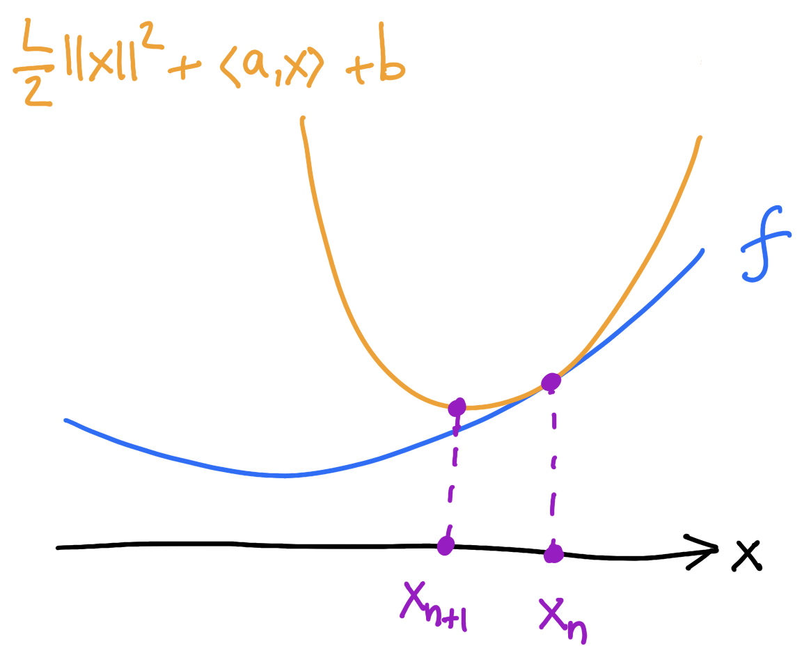
Explicit minimizing movements: warm-up

Two steps: 

1) majorize: find the tangent parabola (“surrogate”)

2) minimize: minimize the surrogate

$$x_{n+1}=x_n-\frac{1}{L}\nabla E(x_n)$$

“Nonsmooth” formulation of Gradient descent:

Warm-up question: how to formulate GD in a nonsmooth context? (ex: metric space)

Explicit minimizing movements: warm-up

Two steps: 

1) majorize: find the tangent parabola (“surrogate”)

2) minimize: minimize the surrogate

If $E$ is $L$-smooth ($\nabla^2 E\leq L I_{d\times d}$) then it sits below the surrogate:

$$E(x)$$

$$\leq$$

$$E(x_n)+\langle\nabla E(x_n),x-x_n\rangle+\frac{L}{2}\lVert x-x_n\rVert^2$$

$$x_{n+1}=x_n-\frac{1}{L}\nabla E(x_n)$$

Explicit minimizing movements: c-concavity

$\exists h\colon Y\to\mathbb{R}\cup\{+\infty\}$

Definition.

$E$ is c-concave if

generalizes “$L$-smoothness”

Abstract setting:

Smallest such $h$ is the c-transform

$h(y)=\sup_{x\in X}E(x)-D(x,y)$

$\exists h\colon Y\to\mathbb{R}\cup\{+\infty\}$

Definition.

$E$ is c-concave if

c-concave

not c-concave

Explicit minimizing movements: c-concavity

Differentiable NNCC setting. Suppose that $\forall x\in X,\exists y\in Y$:  $\nabla_x D(x,y)=\nabla E(x)$ and 

$$\nabla^2 E (x) \leq \nabla^2_{xx}D(x,y).$$

Then $E$ is c-concave. 

Theorem.

(L–Aubin-Frankowski, à la Trudinger–Wang '06)

$\exists h\colon Y\to\mathbb{R}\cup\{+\infty\}$

Definition.

$E$ is c-concave if

Explicit minimizing movements: c-concavity

Explicit minimizing movements

(majorize)

(minimize)

Algorithm.

(Explicit scheme)

Assume $E$ c-concave.

(L–Aubin-Frankowski '23)

Explicit minimizing movements

$X,Y$ smooth manifolds,   $D\in C^1(X\times Y)$,   $E\in C^1(X)$ c-concave

Under certain assumptions, the explicit scheme can be written as

2. Convergence rates

EVI and convergence rates

Definition.

(Csiszár–Tusnády ’84)

(L–Aubin-Frankowski ’23)

Evolution Variational Inequality (or five-point property):

(Ambrosio–Gigli–Savaré ’05)

EVI

Take $X=Y$,   $D\geq 0$,   $D(x,x)=0\,\,\longrightarrow\,\, y_{n+1}=x_n$,

⏵ EVI as a property of $E$:    $\displaystyle \exists x_n  \in\operatorname*{argmin}_{x\in X}E(x)+D(x,x_{n-1})$ s.t.

Ex: $E\colon\R^d\to\R$ $\frac{\mu}{\tau}$-convex,     $D(x,y)=\frac{1}{2\tau}\lVert x-y\rVert^2$

3. A synthetic formulation of nonnegative cross-curvature

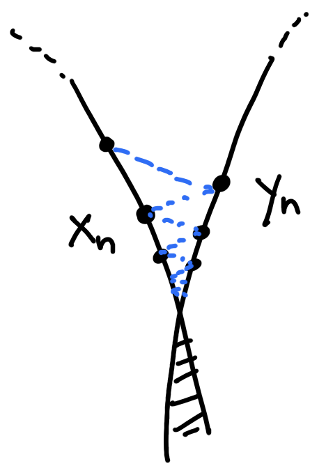
Variational c-segments and NNCC spaces

⏵  $s\mapsto (x(s),\bar y)$ is a variational c-segment if $D(x(s),\bar y)$ is finite and 

⏵  $(X\times Y,D)$ is a space with nonnegative cross-curvature (NNCC space) if variational c-segments always exist.

$X, Y$ two arbitrary sets,   $D\colon X\times Y\to\mathbb{R}\cup\{\pm\infty\}$.

Definition.

(L–Todeschi–Vialard '24)

Origins in regularity of optimal transport

(Ma–Trudinger–Wang ’05)

(Trudinger–Wang ’09)

(Kim–McCann ’10)

convexity of the set of c-concave functions

(Figalli–Kim–McCann '11)

Properties of NNCC spaces

Stable by products

Stable by quotients with “equidistant fibers”

(connect to: Kim–McCann '12)

(L–Todeschi–Vialard '24)

(finite) collection of NNCC spaces $(X^a\times Y^a,c^a)_{a=1..n}$,

$$\mathbf{X}=X^1\times\dots\times X^n,\quad \mathbf{Y}=Y^1\times\dots\times Y^n,\quad \mathbf{c}(\mathbf{x},\mathbf{y})=c^1(x^1,y^1)+\dots+c^n(x^n,y^n)$$

$(\mathbf{X}\times\mathbf{Y},\mathbf{c})$ is NNCC.

$c\colon X\times Y\to [-\infty,+\infty],   P_1\colon X\to\underline{X}$,   $P_2\colon Y\to\underline{Y}$ s.t. “equidistant fibers”

Then: $(X\times Y,c)$ NNCC $\implies$ $(\underline{X}\times\underline{Y},\underline{c})$ NNCC

(connect to: Kim–McCann '12)

Quotients:

Products:

Properties of NNCC spaces

Metric cost $c(x,y)=d^2(x,y)$     NNCC$\implies$PC

(connect to: Ambrosio–Gigli–Savaré ’05)

(connect to: Loeper ’09)

(L–Todeschi–Vialard '24)

Application: transport costs

“Proof.”

 $(X\times Y,c)$   NNCC $\implies$ $(\mathcal{P}(X)\times\mathcal{P}(Y),\mathcal{T}_c)$  NNCC

Ex: $W_2^2$ on $\mathbb{R}^n$, on $\mathbb{S}^n$, OT with Bregman costs...

Variational c-segments $\approx$ generalized geodesics

$X,Y$ Polish,   $c\colon X\times Y\to\R\cup\{+\infty\}$ lsc

1. $(U,V)\mapsto \mathbb{E}\,c(U,V)=\int_\Omega c(U(\omega),V(\omega))\,d\mathbb{P}(\omega)$ is NNCC when $(X\times Y,c)$ is NNCC  “product of NNCC”

2. $\displaystyle\inf_{\operatorname{law}(U)=\mu}\mathbb{E}\,c(U,V)=\inf_{\operatorname{law}(V)=\nu}\mathbb{E}\,c(U,V)=\mathcal{T}_c(\mu,\nu)$     “equidistant fibers” 

Theorem.

(L–Todeschi–Vialard '24)

Examples

Gromov–Wasserstein

Costs on measures. The following are NNCC:

Relative entropy        $\operatorname{KL}(\mu,\nu)=\int \log\Big(\frac{d\mu}{d\nu}\Big)\,d\mu$,

Hellinger                   $D(\mu,\nu)=\displaystyle\int\Big(\sqrt{\frac{d\mu}{d\lambda}}-\sqrt{\frac{d\nu}{d\lambda}}\Big)^2\,d\lambda$,

Fisher–Rao = length space associated with Hellinger

$(\mathbb{G}\times\mathbb{G},\operatorname{GW}^2)$ is NCCC

$\mathbf{X}=[X,f,\mu]$   and   $\mathbf{Y}=[Y,g,\nu]\in\mathbb{G}$

Any Hilbert or Bregman cost is NNCC:

G. Peyré

Convergence rates for minimizing movements

Suppose that for each $x\in X$ and $n\geq 0$,

Then sublinear ($\mu=0$) or linear ($\mu>0$) convergence rates. 

⏵ there exists a variational c-segment $s\mapsto (x(s),y_n)$ on $(X\times Y,D)$ with $x(0)=x_n$ and $x(1)=x$

⏵ $s\mapsto E(x(s))-\mu \,D(x(s),y_{n+1})$ is convex

⏵ $\displaystyle\lim_{s\to 0^+}\frac{D(x(s),y_{n+1})}{s}=0$

Theorem.

(L–Aubin-Frankowski '23)

Thank you!