What I will present

Main motivation: optimization on a space of measures $\mathcal{P}(M)$:

minimize   $E\colon \mathcal{P}(M)\to\mathbb{R}\cup\{+\infty\}$

Typical scheme:

where $D(\mu,\nu)=$

transport cost:   $W_2^2(\mu,\nu)$,  $\mathcal{T}_c(\mu,\nu)$,...

Bregman divergence:   $\operatorname{KL}(\mu,\nu)$,...

Csiszár divergence:   $\int_M (\sqrt{\mu}-\sqrt{\nu})^2$,...

Regularized cost

Minimizing movement schemes based on general movement limiters

...

What I will present

Minimizing movement schemes based on general movement limiters

1. Formulations for implicit and explicit schemes with general movement limiter

→ unify gradient / mirror / natural gradient / Riemannian gradient descents

Implicit scheme

Minimize  $E\colon X\to\mathbb{R}\cup\{+\infty\}$,   where $X$ is a set (finite  or infinite dimensional...)

Use   $D\colon X\times X\to[0,+\infty]$

Motivations for general $D(x,y)$:

Implicit scheme

• $D(x,y)$ tailored to the problem
• Regularized squared distance
• Discretizing gradient flows   “$\dot x(t)=-\nabla E(x(t))$”

Toy example: $\dot x(t)=-\nabla^2u(x(t))^{-1}\nabla E(x(t))$, $u\colon \R^d\to\R$  strictly convex

Two approaches:

$d=$ distance for Hessian metric $\nabla^2 u$

Explicit minimizing movements: warm-up

$$x_{n+1}=x_n-\frac{1}{L}\nabla E(x_n)$$

“Variational” formulation of Gradient descent:

Two steps: 

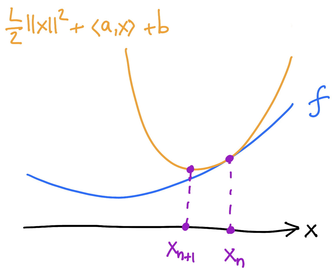
1) majorize: find the tangent parabola (“surrogate”)

2) minimize: minimize the surrogate

Explicit minimizing movements: warm-up

If $E$ is $L$-smooth ($\nabla^2 E\preccurlyeq L I_{d\times d}$) then it sits below the surrogate:

$$E(x)$$

$$\leq$$

$$E(x_n)+\langle\nabla E(x_n),x-x_n\rangle+\frac{L}{2}\lVert x-x_n\rVert^2$$

$$x_{n+1}=x_n-\frac{1}{L}\nabla E(x_n)$$

Two steps: 

1) majorize: find the tangent parabola (“surrogate”)

2) minimize: minimize the surrogate

Explicit minimizing movements: c-concavity

$\exists h\colon Y\to\mathbb{R}\cup\{+\infty\}$

Definition.

$E$ is c-concave if

generalizes “$L$-smoothness”

Abstract setting:

Smallest such $h$ is the c-transform

$h(y)=\sup_{x\in X}E(x)-D(x,y)$

$X,Y$: two sets

$\exists h\colon Y\to\mathbb{R}\cup\{+\infty\}$

Definition.

$E$ is c-concave if

c-concave

not c-concave

Explicit minimizing movements: c-concavity

Suppose that $\forall x\in X,\exists y\in Y$:  $\nabla_x D(x,y)=\nabla E(x)$ and $\nabla^2 E (x) \leq \nabla^2_{xx}D(x,y).$

Then $E$ is c-concave. 

$\exists h\colon Y\to\mathbb{R}\cup\{+\infty\}$

Definition.

$E$ is c-concave if

Explicit minimizing movements: c-concavity

$E$ is c-concave $\iff \nabla^2 E\preccurlyeq L\, I_{d\times d}$

Example.

Example.

Differentiable NNCC setting.

Explicit minimizing movements

(majorize)

(minimize)

Algorithm.

(Explicit scheme)

Assume $E$ c-concave.

(L–Aubin-Frankowski '23)

Other point of view:

Explicit minimizing movements

$X,Y$ smooth manifolds,   $D\in C^1(X\times Y)$,   $E\in C^1(X)$ c-concave

Under certain assumptions, the explicit scheme can be written as

2. Convergence rates

EVI and convergence rates

Definition.

(Csiszár–Tusnády ’84)

(L–Aubin-Frankowski ’23)

Evolution Variational Inequality (or five-point property):

(Ambrosio–Gigli–Savaré ’05)

Variational c-segments and NNCC spaces

⏵  $s\mapsto (x(s),\bar y)$ is a variational c-segment if $D(x(s),\bar y)$ is finite and 

⏵  $(X\times Y,D)$ is a space with nonnegative cross-curvature (NNCC space) if variational c-segments always exist.

$X, Y$ two arbitrary sets,   $D\colon X\times Y\to\mathbb{R}\cup\{\pm\infty\}$.

Definition.

(L–Todeschi–Vialard '24)

Origins in regularity of optimal transport

(Ma–Trudinger–Wang ’05)

(Trudinger–Wang ’09)

(Kim–McCann ’10)

convexity of the set of c-concave functions

(Figalli–Kim–McCann '11)

Finite dimensional examples

$D(x,y)=$ Bregman divergence on $\mathbb{R}^d$

$D(x,y)=\lVert x-y\rVert^2$ on $\mathbb{R}^d$

Sphere $\mathbb{S}^d$ with the squared geodesic distance

Bures–Wasserstein

Infinite dimensional examples

Gromov–Wasserstein

Costs on measures. The following are NNCC:

Relative entropy        $\operatorname{KL}(\mu,\nu)=\int \log\Big(\frac{d\mu}{d\nu}\Big)\,d\mu$,

Hellinger                   $D(\mu,\nu)=\displaystyle\int\Big(\sqrt{\frac{d\mu}{d\lambda}}-\sqrt{\frac{d\nu}{d\lambda}}\Big)^2\,d\lambda$,

Fisher–Rao = length space associated with Hellinger

Transport costs: squared Wasserstein distance on $\R^d$, on the sphere...

$(\mathbb{G}\times\mathbb{G},\operatorname{GW}^2)$ is NCCC

$\mathbf{X}=[X,f,\mu]$   and   $\mathbf{Y}=[Y,g,\nu]\in\mathbb{G}$

G. Peyré

Convergence rates for minimizing movements

Suppose that for each $x\in X$ and $n\geq 0$,

Then sublinear ($\mu=0$) or linear ($\mu>0$) convergence rates. 

⏵ there exists a variational c-segment $s\mapsto (x(s),y_n)$ on $(X\times Y,D)$ with $x(0)=x_n$ and $x(1)=x$

⏵ $s\mapsto E(x(s))-\mu \,D(x(s),y_{n+1})$ is convex

⏵ $\displaystyle\lim_{s\to 0^+}\frac{D(x(s),y_{n+1})}{s}=0$

Theorem.

(L–Aubin-Frankowski '23)

3. Applications

Background on mirror descent

Minimize $E\colon\R^d\to\R$   without using the Euclidean structure

Instead use strictly convex $u\colon\R^d\to\R$.

“Mirror map” $\nabla u\colon\R^d\to\R^d$ to go from primal to dual space

Mirror descent

Convergence rates: if $\mu\nabla^2u\preccurlyeq\nabla^2E\preccurlyeq\nabla^2u$ then

Nondifferentiable mirror descent

Idea: cost $D(x,y)=u(x)+u^*(y)-\langle x,y\rangle=u(x|\tilde y)$      for $y=\nabla u(\tilde y)$

$X=Y=\mathbb{R}^d$, $u\colon \mathbb{R}^d\to\mathbb{R}\cup\{+\infty\}$ convex

Given $y_n$,

$E\colon \mathbb{R}^d\to\mathbb{R}\cup\{+\infty\}$

Assume $E$ convex and $u-E$ convex

Convergence rate:

Algorithm.

Theorem.

$D(x,y)=u(y|x)\longrightarrow$ $x_{n+1}-x_n=-\nabla^2u(x_n)^{-1}\nabla f(x_n)$

If $$\nabla^3u(\nabla^2u^{-1}\nabla f,-,-)\leq \nabla^2f\leq \nabla^2u+\nabla^3u(\nabla^2u^{-1}\nabla f,-,-)$$ then

$$f(x_n)\leq f(x)+\frac{u(x_0|x)}{n}$$

Global rates for Newton's method

Riemannian setting

da Cruz Neto, de Lima, Oliveira ’98

Bento, Ferreira, Melo ’17

2. Explicit:    $x_{n+1}=\exp_{x_n}\big(-\tau\nabla f(x_n)\big)$

    $\operatorname{Riem}\geq 0$: $\nabla^2f\geq 0$ gives $O(1/n)$ convergence rates

    $\operatorname{Riem}\leq 0$: convexity of $f$ on c-segments gives $O(1/n)$ convergence rates

1. Implicit:     $x_{n+1}=\argmin_{x} f(x)+\frac{1}{2\tau}d_M^2(x,x_n)$

    $\operatorname{Riem}\leq 0$: $\nabla^2f\geq 0$ gives $O(1/n)$ convergence rates

$\operatorname{Riem}\geq 0$: convexity of $f$ on c-segments gives $O(1/n)$ convergence rates

Thank you!