Dimentionality reduction and classification over MRI anatomical images using PCA
What is Dimensionality Reduction?
- Too many features while the availability of training examples is not infinite
E.g. 3D Image processing 256*256*256 = 16777216 features
- As the number of feature or dimensions grows, the amount of data we need to generalise accurately grows exponentially.
- Sometimes, most of these features are correlated and hence redundant
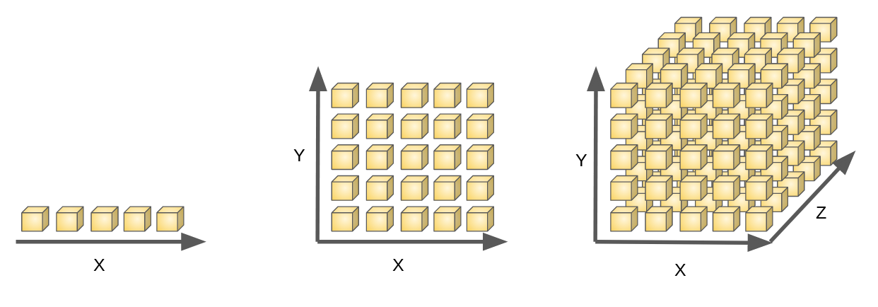
- Feature selection & Feature extraction
Avoid curse of dimensionality:
- Reduce computational time and space required
- Ease of fitting models with high accuracy (bye to over-fitting)
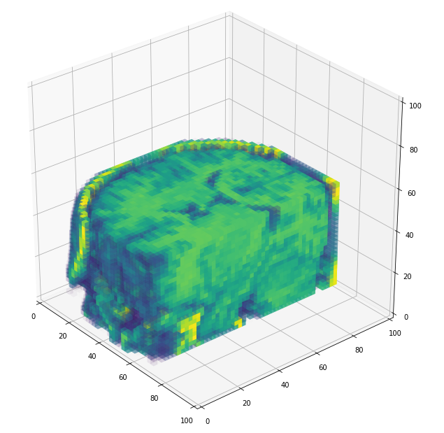
- Possibility to visualize the data when reduced to 2D or 3D
Some dimensionality reduction techniques:
- ICA (independent source finding)
- SVD (efficient computation of PCA)
- PCA (correlated variables to linearly uncorrelated variables)
Why dimensionality reduction...
Data & Data Structure
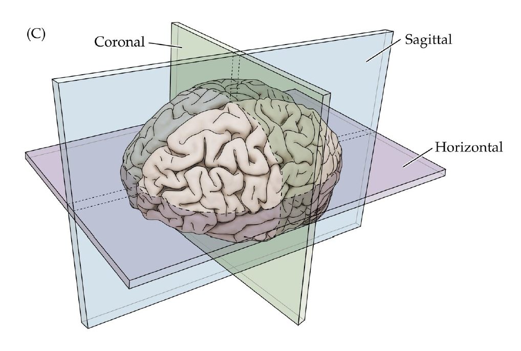
- MRI brain images (volumetric representation)
- NIfTI (.nii) files
- Size: 17.3 GB
- 1113 samples (brains)
- Preprocessed version of data
- Skull stripping.
- Normalized.
The human connectome project, 1113 subjects’ brain T1w structural images. These 3D MPRAGE (this sounds nice) images obtained from Siemens 3T platforms using a 32-channel head coil.

Cropping
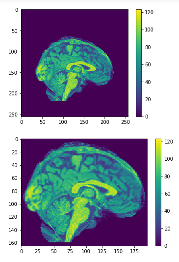
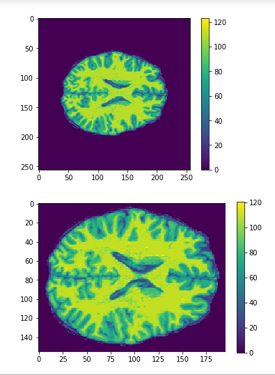
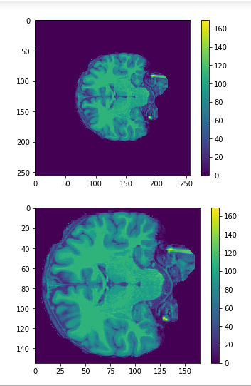
cropped = data[50:205,60:225,30:225] #155x165x195
data = img.get_data() #256x256x256
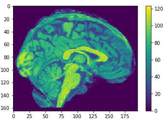
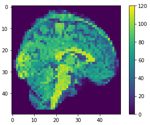
Resize
(155, 165, 195) array  #4987125 voxels
(50, 50, 50) array #125000 voxels
resampled = zoom(cropped, (50/cropped.shape[0], 50/cropped.shape[1] , 50/cropped.shape[2])
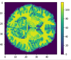
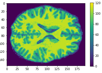
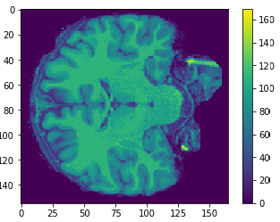
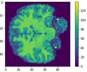
Flatten
(50, 50, 50) array #125000 voxels
vector = array.flatten()
(125000)array #125000 voxels
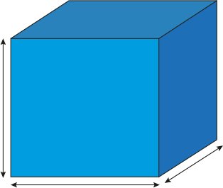


256x256x256
155x165x195
50x50x50
Original
Cropped
Resized
50x50x50
1113x125000
Save
1113 x 125000


1113
1
Flatten

file.npy
jupyter notebook
Loading, cropping , resizing and saving
Principal Component Analysis
(PCA)
What is PCA
- Finding correlation between variables.
- Separating samples on a dataset.
- Eigenvalues and eigenvectors (axes of subspace)
Principal Component Analysis (PCA) is a dimension-reduction tool that can be used to reduce a large set of variables to a small set that still contains most of the information in the large set.
Visually

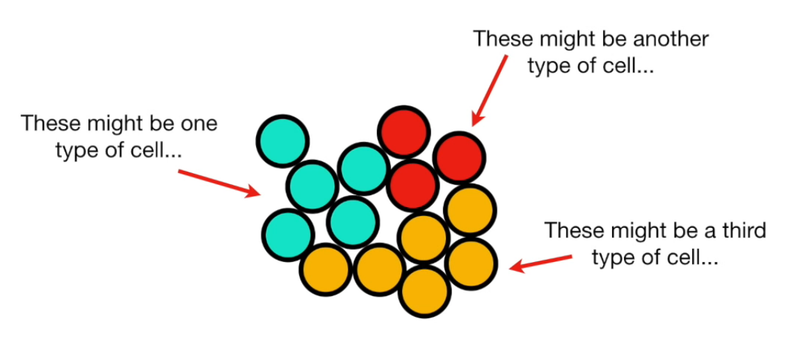
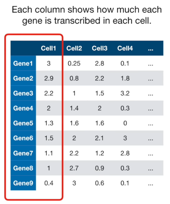
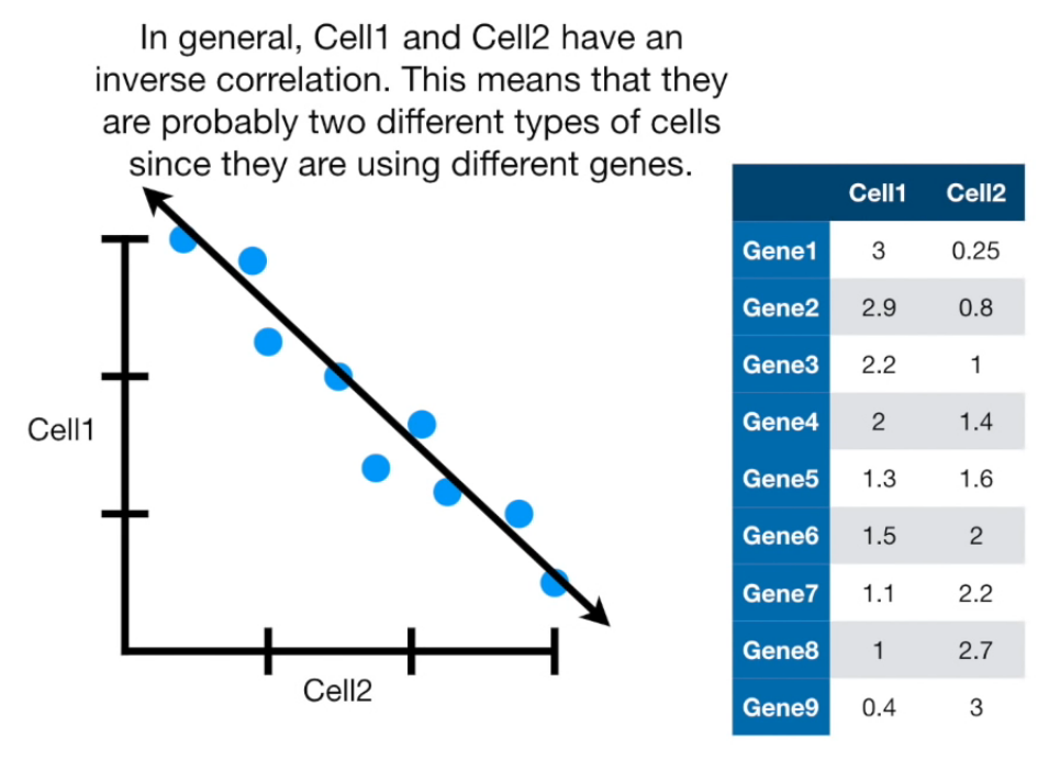
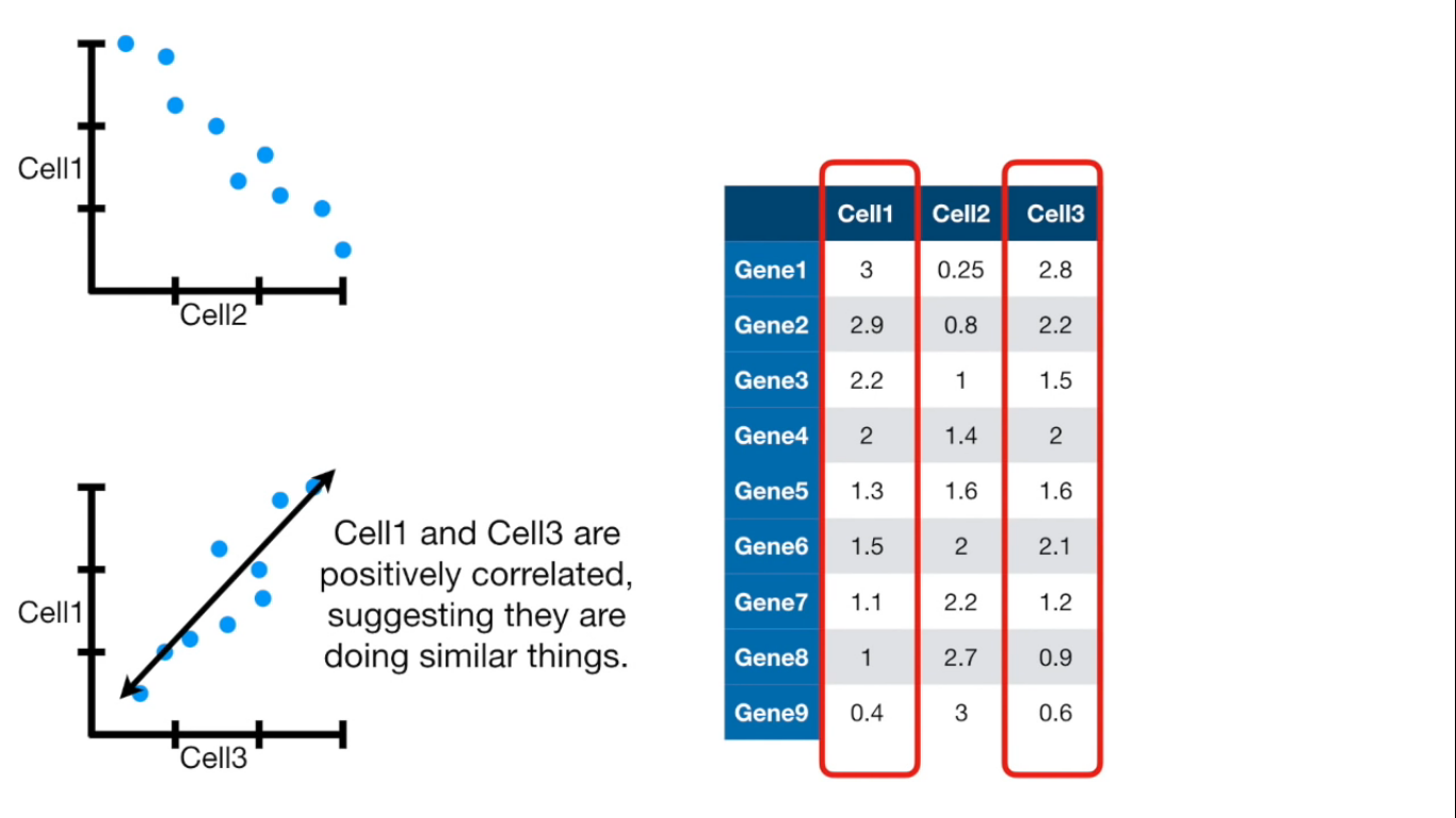
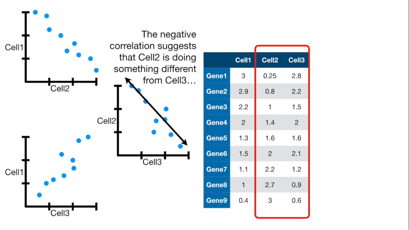
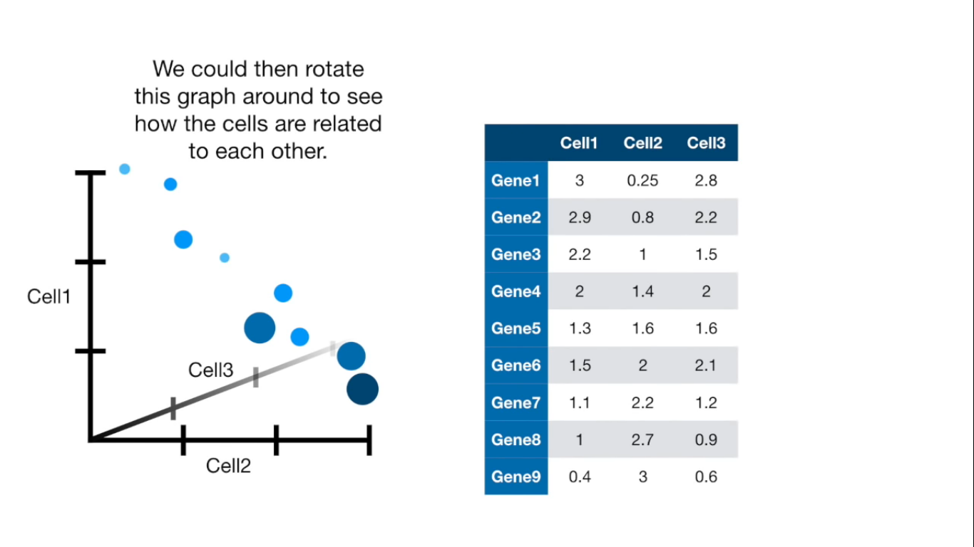
If more than 4 columns...
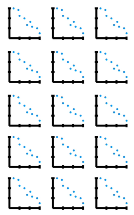
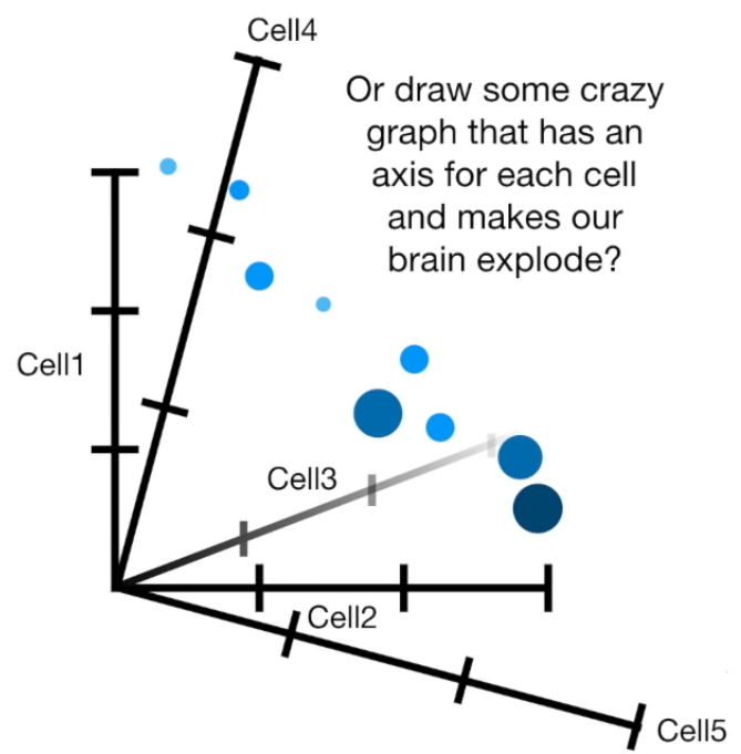
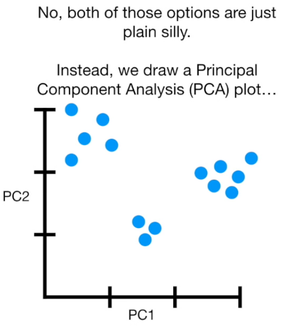
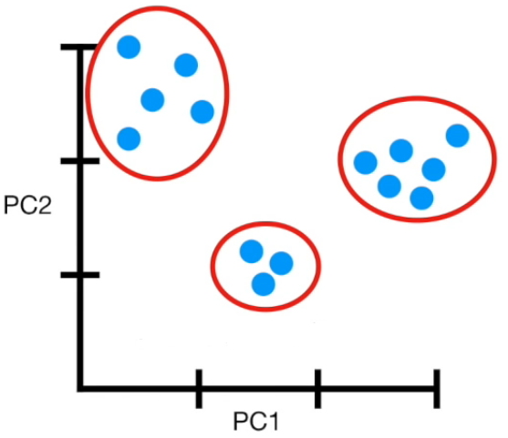
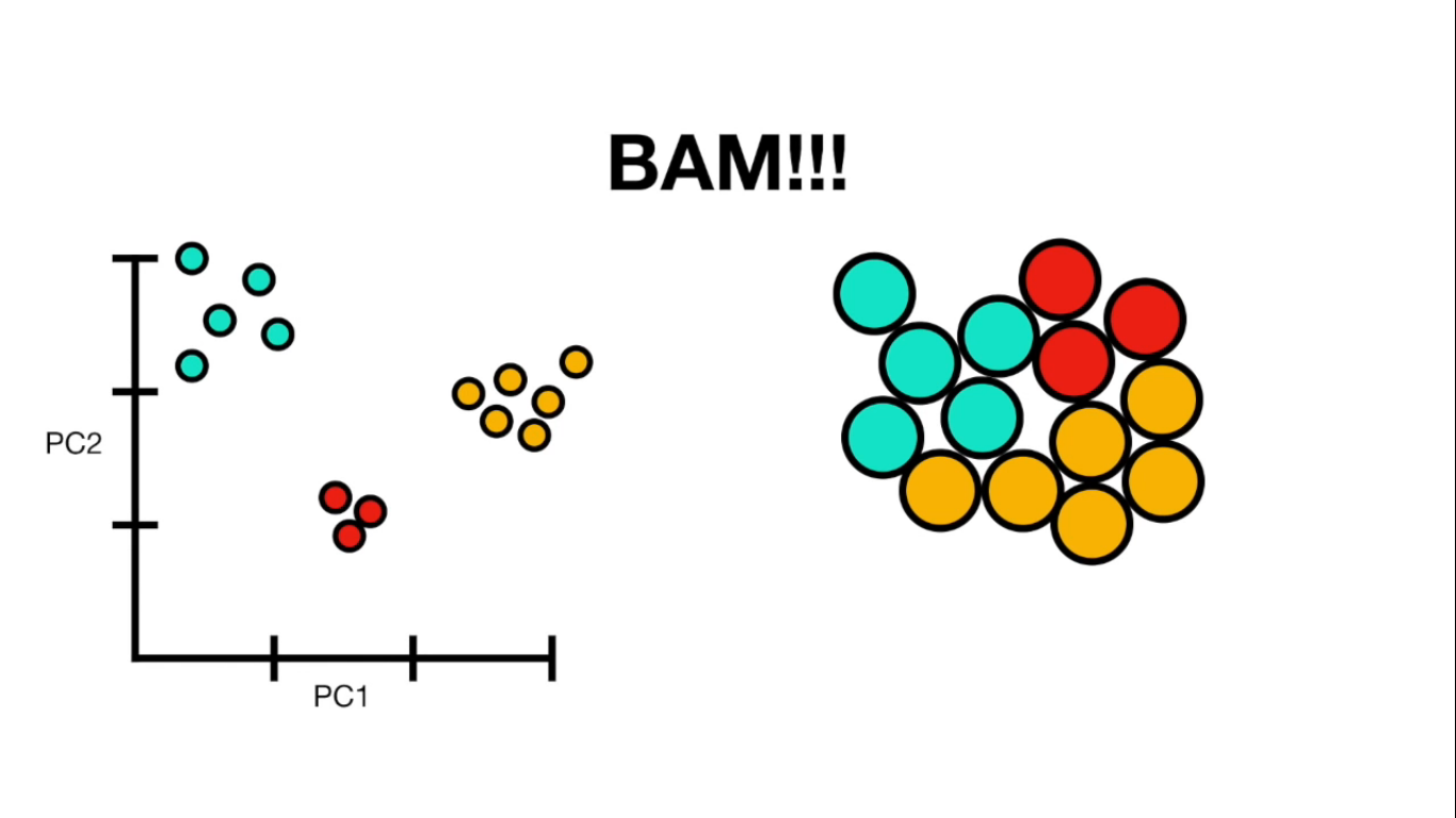
- PCA(1113x125000)
Reduce the amount of features from the original data to a serie of principal components that hold the information of the variance (axis of subspace)
EigenBrains
- (PCA(125000x1113))
Try to find a set of "standardized brain ingredients".
Feature extraction
Feature extraction
- Loading data
- Applying PCA choosing amount of components
- Plotting
- Reconstructing data from components
import numpy as np
to_save_load=np.load("to_save.npy")
to_save_load.shape
(1113, 125000)
Loading data
from sklearn.decomposition import PCA
pca = PCA(n_components=10)#% of variance or number
principalComponents = pca.fit_transform(to_save_load)
(1113, 10)
Applying PCA

l = pca.explained_variance_ratio_
sum(l)#0.412558136188802
Plotting
import pandas as pd
subjects = pd.read_csv('subjects.csv')
columns = subjects[['Subject','class']]
labels= columns.set_index('Subject').T.to_dict('list')
import os
dirs = os.listdir( "brain_nii" )
-
Getting Colors
{585256: [-1], 585862: [-1], 586460: [-1], 587664: [-1], 588565: [1],...}
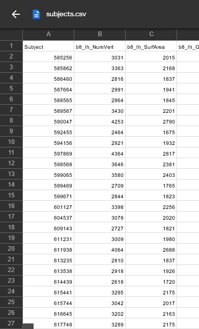
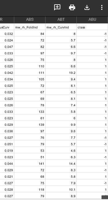
colors = []
for name in dirs:
id,ext = name.split('.')
try:
colors.append(labels[int(id)][0])
except:
colors.append(0)
[1, -1, 1, 1, 1, 1, 1, 1, -1, 1, -1, -1, 1, 1,...] #1 ,0(unlabeled) ,-1
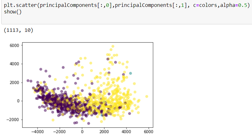
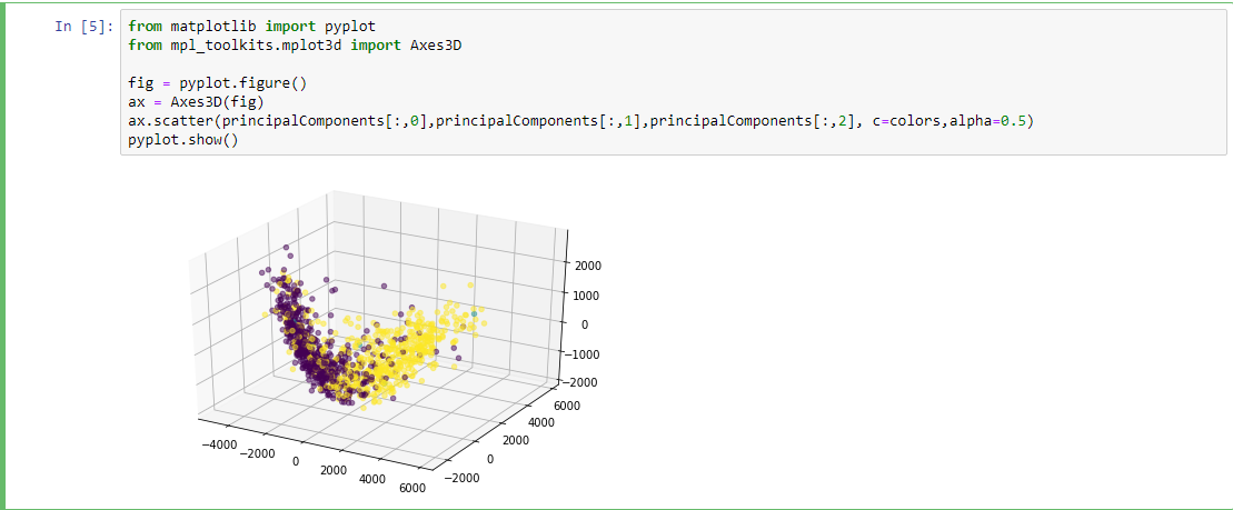
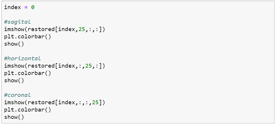
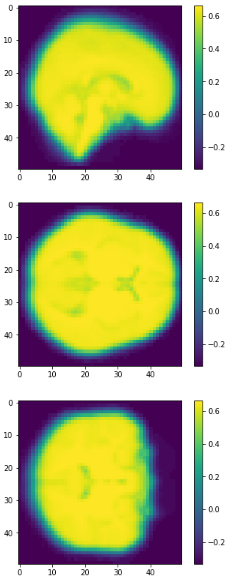
Data reconstruction
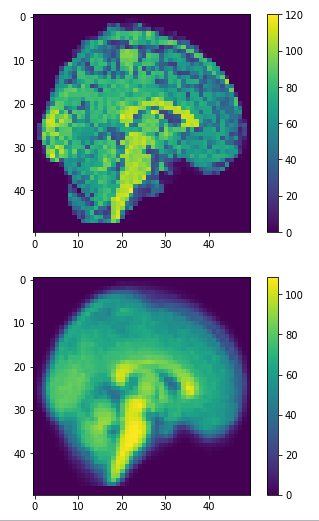
dim=50
approximation = pca.inverse_transform(principalComponents)
restored = approximation.reshape(-1,dim,dim,dim)
(1113, 50,50,50)
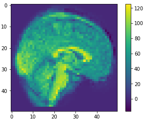
10
100
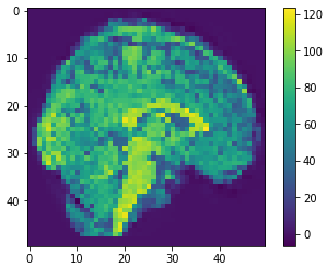
500
0.41
0.81
0.59
Eigen brains
- What is an Eigen brain
- Applying PCA
- Plotting
EigenBrains??
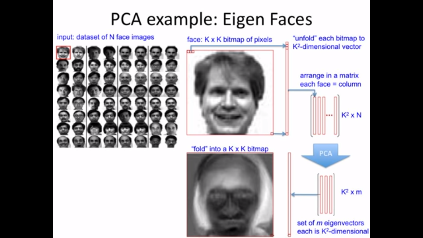

Applying PCA
1113x125000
125000x1113
125000x809
Transpose
PCA(99.9)
Reshaping

125000x809
Transpose
Reshape
50x50x50


eigen brain 809
eigen brain 1
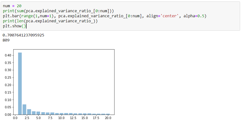
Plotting
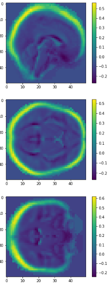
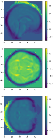

0.417
0.069
0.035
0.022
1
2
3
4
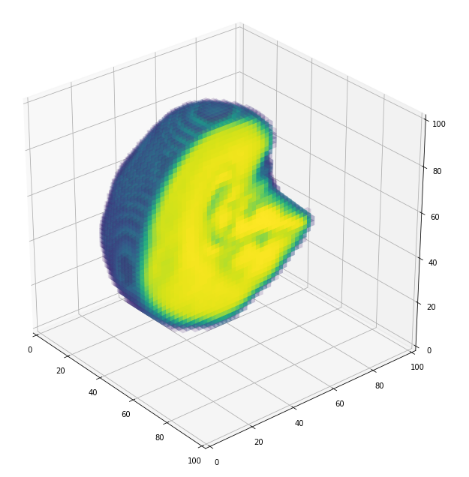
3D volume (fail)
jupyter notebook
PCA , Eigen brains
Classification
- Data pre-processing
- a bit more about the data.
- Resampling and hyperparameter tunning
- cross validation
- testing with different parameter values
- Models fittings
- underfitting and overfitting
- convergence
Post-PCA Data Proprocessing
After PCA:
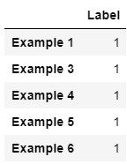
- Data set of dimension 1113x1062 ('PCA.npy')
- Data in the form of array (npy format)
Clasification
- Data label of dimension 1113x1 ('Y.npy')
- Label 1 represents positive brains
- Label -1 represent negative brains
- Label 0 represent unlabeled brains
Post-PCA Data Proprocessing
Post-PCA Data Proprocessing
-Store the index of unlabeled examples & Remove them from the data set
-Replace examples of label -1 with 0 for classification training process (it is better to change to dummy label 0 and 1)
-Concatenate data set with the corresponding labels, rename the columns as PCA1, PCA2,....,PCA1062,CLASS
Post-PCA Data Proprocessing After PCA: Data set of dimension 1113x1062 ('PCA.npy') Data in the form of array (npy format) Clasification


Post-PCA Data Proprocessing
- Data label of dimension 1113x1 ('Y.npy')
- Label 1 represents positive brains
- Label -1 represent negative brains
- Label 0 represent unlabeled brains
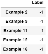
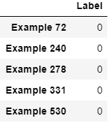
Cleaning data
- Remove unlabeled data
- Change labels
- Concatenate data vs labels
- Evenly distribute data
Load Data & label data
(Remove unlabeled samples from the data set)
data=pd.DataFrame(np.load('PCA.npy'))
y=np.load('Y.npy')
y=pd.DataFrame(y)
dataset=pd.concat([data,y],axis=1)
index_remove=list(y[y[0]==0].index)
print(index_remove)
dataset=dataset.drop(index_remove)
[71, 239, 277, 330, 529]
Cleaning data
Replace examples of label -1 with 0 for classification training process (it is better to change to dummy label 0 and 1)
dataset['class'].replace(-1,0,inplace=True)


Cleaning data
Change labels
Rename the columns as PCA1, PCA2,....,PCA1062,CLASS
a=['PCA' + str(i+1) for i in range(1063)]
a[-1]='CLASS'
dataset.columns=a
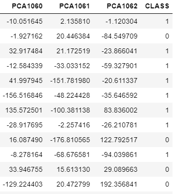
Cleaning data
Evenly distribute data
Problem: Dataset is organized by example labels
class1 = dataset[(dataset['CLASS']== 1)]
print("Total class 1:", len(class1))
class0 = dataset[(dataset['CLASS']== 0)]
print("Total class 0:", len(class0))
df = []
for i in range(550):
df.append(class1.iloc[i].values)
df.append(class0.iloc[i].values)
for j in range(550,558):
df.append(class0.iloc[i].values)


class1 = dataset[(dataset['class']== 1)]
class2 = dataset[(dataset['class']== 0)]

Final processed data
np.save('X_y.npy',df)
- Save the processed data in .npy
- Load the final data
data=pd.DataFrame(np.load('X_y.npy'))
data.iloc[:,-1]=data.iloc[:,-1].apply(lambda i: int(i))
- Assign value to independent and dependent variables
y=np.array(data.iloc[:,-1].replace(-1,0)).ravel()
X=np.array(data.iloc[:,:-1])
Resampling Methods
The process of repeatedly drawing samples from data and refitting a given model on each sample
Resampling methods help:
- Learn more about the fitted model
- Estimates more accurately the error or accuracy for future data
- Estimates the bias and standard deviation of the hypothesized parameters
- Avoids over-fitting
But:
- Computationally expensive
- Underestimate or overestimate the real error
Resampling Methods
Techniques:
- Cross Validation
+ Validation set
+ Leave-one-out cross-validation (LOOCV)
+ K-fold cross validation
-
The Bootstrap
Resampling Methods
Validation Set
- Training data (70%): fitting purpose
- Validation set (20%): how good is the model for future data
- Test set (10%): generalization
train_percentage = 0.7
validation_percentage = 0.2
test_percentage = 0.1
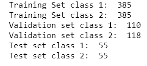
1108 examples
Resampling Methods
Validation Set
Problem: High bias and variability in error/accuracy between the splits.
E.g. For Support Vector Machine using Linear Kernel
Random split 1:
Random plit 2:
Random split 3:


The result highly dependent on 1 split is potentially biased
Resampling Methods
Leave-one-out cross-validation (LOOCV)
Leave-one-out cross-validation withholds only a single observation for the validation set.
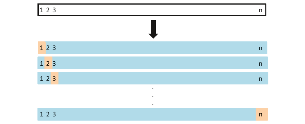
Okay, for our data set, at least 1103 times the model is fit!!!
Resampling Methods
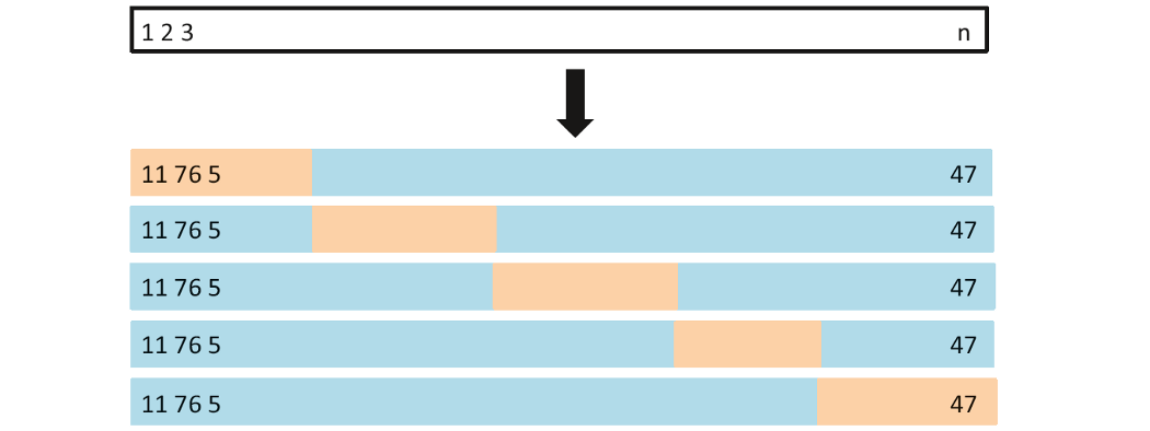
K-fold cross validation
- The technique that randomly divides the whole data set into k subsets, groups or folds (k can be freely chosen)
- Each of k folds can be used as test set while other k-1 folds as training set.
Resampling Methods
K-fold cross validation
Advantage:
- Less computationally expensive
- More accurate estimation for future data
- Easy to apply
- Applicable to large data
Disadvantage:
- Prone to underestimation of real error/overestimation of accuracy
- Not really effective for small data set
K-fold cross validation
from sklearn.model_selection import KFold
kf = KFold(n_splits=5)
kf.get_n_splits(X)

for train_index, test_index in kf.split(X): train_index
test_index


K-fold cross validation
Assign train_index,test_index to form
- X_train, y_train
- X_test, y_test
for train_index, test_index in kf.split(X):
X_train, X_test = X[train_index], X[test_index]
y_train, y_test = y[train_index], y[test_index]
Model fittings
- Logistic Regression using Regularization method (Ridge regression)
- Support Vector Machine with Linear Kernel
- Support Vector Machine with Gaussian Kernel
- K-nearest neighbors (k-nn)
- Neural Network
Model fittings
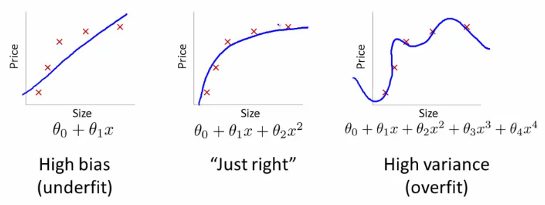
Problems: Over-fitting vs Under-fitting
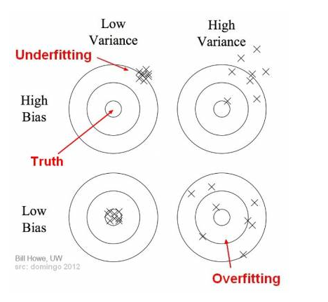
Bias:
- how closeness is our predictive model’s to training data
- very little attention to the training data and oversimplifies the model
=>high error on training and test data
Variance:
- variability of model prediction for a given data point or a value showing spread of our data
- a lot of attention to training data and does not generalize on new data
=> perform very well on training data but badly on test data
Model fittings
Underfitting happens when a model unable to capture the underlying pattern of the data => high bias, low variance
Overfitting happens when model captures the noise along with the underlying pattern in data. In other words, our model is trained a lot over noisy data => low bias, high variance
Model fittings
Why over-fitting:
- Too complex models, too many features
- Too small training data set
- Too small regularization term
...
Why under-fitting:
- Too simple model while the data are too complex
- Too large regularization term
Model fittings
Logistic Regression
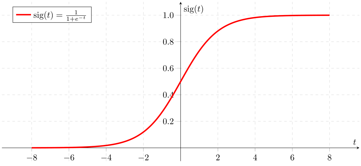
- Also called Sigmoid Function
- In classification problem, the models should better output the prediction values over (0,1) => no sense for predicted values > 1 or < 0
E.g. 0 as non-spam email
1 as spam email
- Sometimes, linear regression does not work well (classification is not actually a linear function)
=> binary classification problem
Logistic Regression
Apply Sigmoid or Logistic Function

where:

Hypothesis or predicted output:


Logistic Regression
Cost function
To address overfitting as our dataset includes up to 1062 features
=> L1 Regularization term added
Logistic Regression using Regularization (Ridge regression)

Note:
Too large lambda could lead to under-fitting
Too small lambda could keep the model still over-fitting
Logistic Regression
Apply Logistic Regression
from sklearn.linear_model import LogisticRegression
def log_reg(X_train,X_test,y_train,y_test,reg_term):
classifier = LogisticRegression(solver='liblinear',penalty='l1',C=(1/reg_term),fit_intercept=True,max_iter=500)
classifier.fit(X_train,y_train)
return classifier.score(X_train,y_train),classifier.score(X_test,y_test)
Return the accuracy rate of the model over training and test set
Note:
C=1/(regularization term)
Logistic Regression
Define the best regularization term "lambda" for logistic regression model using cross validation
Number of folds: k=5
kf = KFold(n_splits=5)
List of regularization term :
param_logreg=[0.001*10**i for i in range(10)]

Logistic Regression
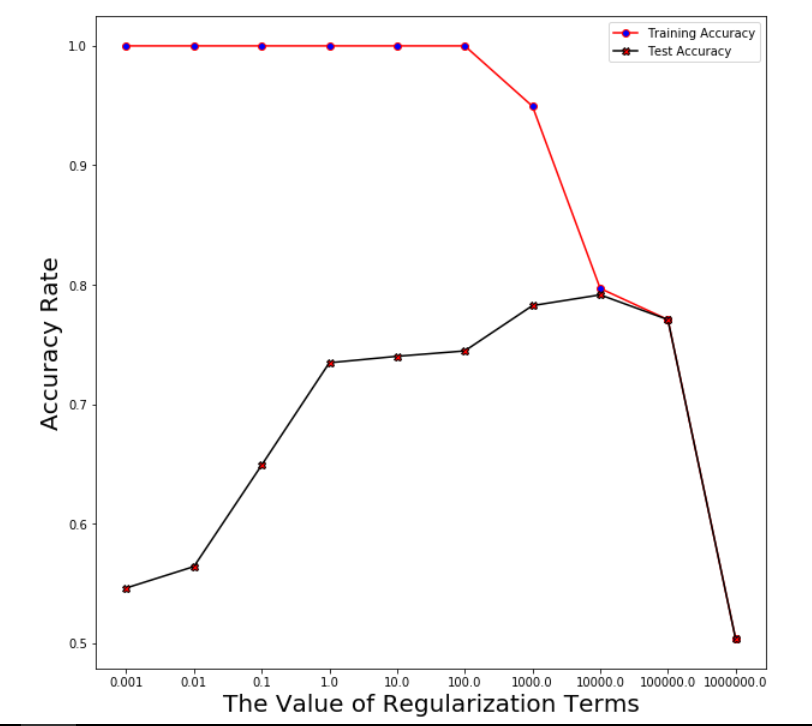
Step 1: find the best range with the best performance over both training and test set
training_acc_col=[]
test_acc_col=[]
for train_index, test_index in kf.split(X):
training_acc_col.append([])
test_acc_col.append([])
X_train, X_test = X[train_index], X[test_index]
y_train, y_test = y[train_index], y[test_index]
for i in param_logreg:
training_acc,test_acc=log_reg(X_train,X_test,y_train,y_test,i)
training_acc_col[-1].append(training_acc)
test_acc_col[-1].append(test_acc)
Logistic Regression
Plot averaged training accuracy & test accuracy over the range of regularization terms after running through 5 folds
x_i=[i for i in range(len(param_logreg))]
plt.figure(figsize=(10,10))
plt.plot(x_i,avg_training_acc,marker='o',mfc='blue',color='r')
plt.plot(x_i,avg_test_acc,marker='X',mfc='red',color='black')
plt.xticks(x_i,param_logreg)
plt.legend(['Training Accuracy','Test Accuracy'])
plt.xlabel('The Value of Regularization Terms',size=20)
plt.ylabel('Accuracy Rate',size=20)
plt.show()
avg_training_acc=np.mean(np.array(training_acc_col),axis=0)
avg_test_acc=np.mean(np.array(test_acc_col),axis=0)
Logistic Regression
Logistic Regression
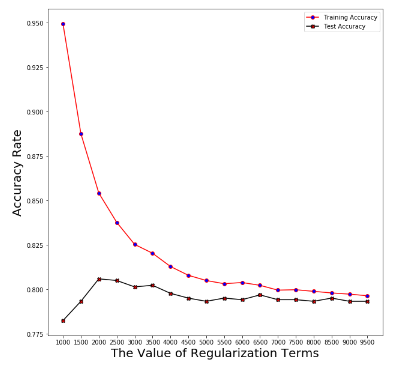
Step 2: Find the exact value of the best regularization term (we choose from 1000 to 10000)
param_logreg=[]
training_acc_col=[]
test_acc_col=[]
for i in range(1000,10000,500):
param_logreg.append(i)
for train_index, test_index in kf.split(X):
training_acc_col.append([])
test_acc_col.append([])
X_train, X_test = X[train_index], X[test_index]
y_train, y_test = y[train_index], y[test_index]
for i in param_logreg:
training_acc,test_acc=log_reg(X_train,X_test,y_train,y_test,i)
training_acc_col[-1].append(training_acc)
test_acc_col[-1].append(test_acc)
Logistic Regression
Plotting the averaged accuracy
avg_training_acc=np.mean(np.array(training_acc_col),axis=0)
avg_test_acc=np.mean(np.array(test_acc_col),axis=0)
x_i=[i for i in range(len(param_logreg))]
plt.figure(figsize=(10,10))
plt.plot(x_i,avg_training_acc,marker='o',mfc='blue',color='r')
plt.plot(x_i,avg_test_acc,marker='X',mfc='red',color='black')
plt.xticks(x_i,param_logreg)
plt.xlabel('The Value of Regularization Terms',size=20)
plt.ylabel('Accuracy Rate',size=20)
plt.legend(['Training Accuracy','Test Accuracy'])
# plt.xlim(min(param_logreg)/10,max(param_logreg))
plt.show()
Logistic Regression
Logistic Regression
Regularization term: log_reg_term=2500
Averaged training accuracy: 83.78%
Averaged test accuracy: 80.51%
Support Vector Machine
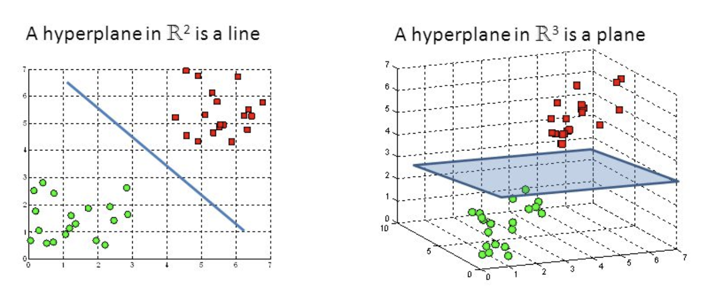
- A discriminative classifier formally defined by a separating hyperplane
- The algorithm outputs an optimal hyperplane which categorizes new examples (a line in 2-D dimension)
Support Vector Machine
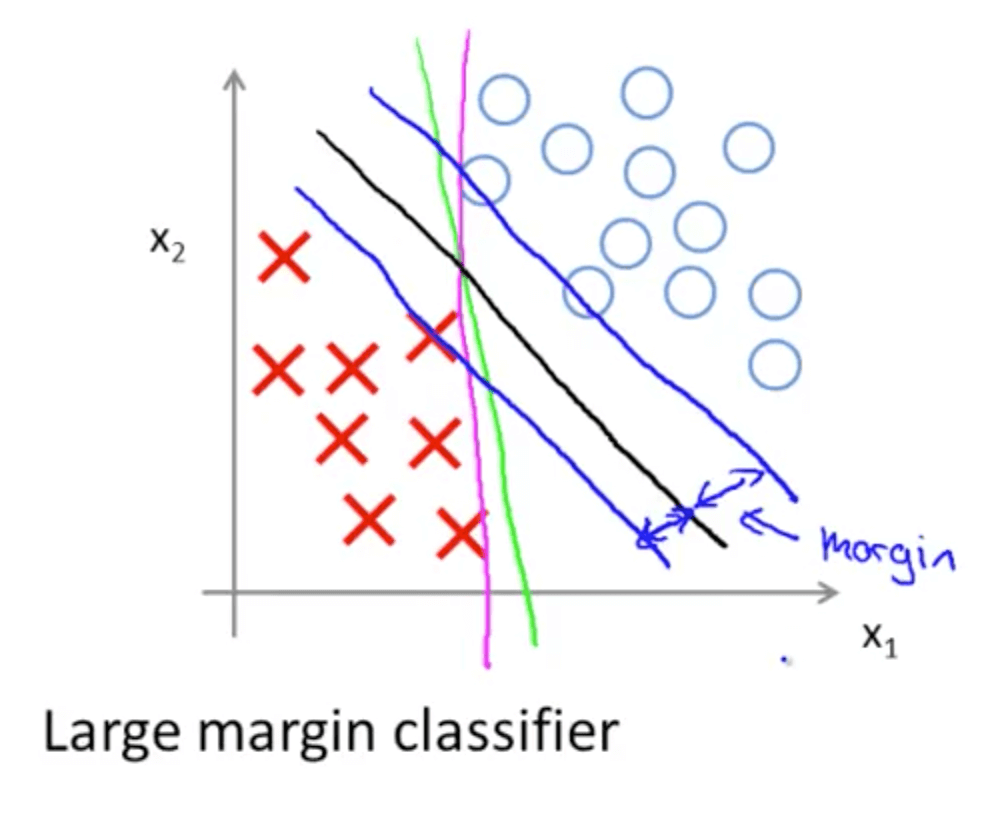
Support Vector Machine

Cost Function

Objective Function
If C=(1/lambda), SVM with linear kernel and Logistic Regression using regularization give exactly the same hypothesized parameters
C too large: over-fitting
C too small: under-fitting
Instead of A + λB, we use CA + B
Support Vector Machine
kf = KFold(n_splits=5)
Applying Support Vector Machine with Linear Kernel
Number of folds (iterations): k=5
List of regularization terms:

=> Define the best regularization term
Support Vector Machine
Define the best range of regularization terms
training_acc_col=[]
test_acc_col=[]
for train_index, test_index in kf.split(X):
training_acc_col.append([])
test_acc_col.append([])
X_train, X_test = X[train_index], X[test_index]
y_train, y_test = y[train_index], y[test_index]
for i in param_linear_svc:
training_acc,test_acc=linear_svc(X_train,X_test,y_train,y_test,i)
training_acc_col[-1].append(training_acc)
test_acc_col[-1].append(test_acc)
Support Vector Machine
Plotting the averaged training and test error after running through 5 folds
avg_training_acc=np.mean(np.array(training_acc_col),axis=0)
avg_test_acc=np.mean(np.array(test_acc_col),axis=0)
x_i=[i for i in range(len(param_linear_svc))]
plt.figure(figsize=(10,10))
ax = plt.subplot(111)
plt.plot(x_i,avg_training_acc,marker='o',mfc='blue',color='r')
plt.plot(x_i,avg_test_acc,marker='X',mfc='red',color='black')
xlabel=['10^'+str(i) for i in range(3,13)]
plt.xticks(x_i,xlabel)
plt.xlabel('The Value of Regularization Terms',size=20)
plt.ylabel('Accuracy Rate',size=20)
plt.show()
Support Vector Machine
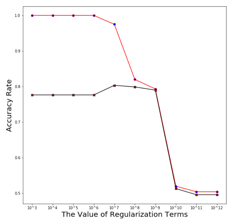
Support Vector Machine
Find the exact value of the best regularization term (we choose from C = 10^7 to 10^8)
training_acc_col=[]
test_acc_col=[]
param_linear_svc=[i for i in range(10**7,10**8+1,int((10**7)))]
print('Regularization terms:',param_linear_svc)
for train_index, test_index in kf.split(X):
training_acc_col.append([])
test_acc_col.append([])
X_train, X_test = X[train_index], X[test_index]
y_train, y_test = y[train_index], y[test_index]
for i in param_linear_svc:
training_acc,test_acc=linear_svc(X_train,X_test,y_train,y_test,i)
training_acc_col[-1].append(training_acc)
test_acc_col[-1].append(test_acc)
Support Vector Machine
Plotting the averaged training and test error after running through 5 folds
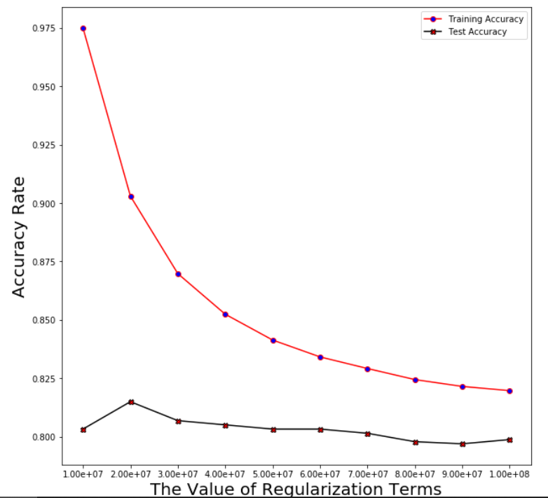
Support Vector Machine
Regularization linear_svc_reg=3*10**7
Averaged training accuracy: 86.98%
Averaged test accuracy: 80.69%
Support Vector Machine
with Gaussian Kernel
Gaussian kernel a function whose value depends on the distance from the origin or from some point.
Conclusions
- It is possible to reduce the dimension using simple operations like: cropping and resizing , however, this also means we lose information.
- PCA help us reduce the amount of features by finding a subspace in which classes can be seperated normally using the principal components as new axes for our data.
- PCA can be used for different purposes depending the application.
- The computation of PCA is fairly expensive and can be speeded up by using SVD algorithm.
- Vizualization of volumes is expensive...(GPU based solutions)
dimentionality redution over
By gabriel munoz
dimentionality redution over
- 292


