FROM CODE TO LIGHT
USING MACHINE LEARNING AND OPTIMIZATION TECHNIQUES TO DESIGN PHOTONIC NANOSTRUCTURES
Giovanni Pellegrini
OUTLINE OF THE TUTORIAL
-
The problem
-
The software tools
-
A bit of theory
-
Handling the data
-
Training the forward model
-
Training the inverse model
THE NOTEBOOKS AND THESE SLIDES


Data analysis
Direct model
Inverse model

These slides
A "TOY" PROBLEM FOR OUR TUTORIAL
OPTICAL PROPERTIES OF NANOHOLE ARRAYS
Eosam 2024, 9-13 September 2024, Naples

Jahan, T. et al. Deep learning-driven forward and inverse design of nanophotonic nanohole arrays: streamlining design for tailored optical functionalities and enhancing accessibility. Nanoscale (2024) doi:10.1039/D4NR03081H.

A "TOY" PROBLEM FOR OUR TUTORIAL
OPTICAL PROPERTIES OF NANOHOLE ARRAYS
| n.1 | n.2 | n.3 | |
|---|---|---|---|
| Lattice | Hexagonal | Square | Square |
| Material | Ag | Au | SiOx |
| Thickness (nm) | 100 | 115 | 90 |
| Radius (nm) |
60 | 110 | 140 |
| Pitch (nm) |
450 | 550 | 515 |

DIRECT
INVERSE
Jahan, T. et al. Deep learning-driven forward and inverse design of nanophotonic nanohole arrays: streamlining design for tailored optical functionalities and enhancing accessibility. Nanoscale (2024) doi:10.1039/D4NR03081H.
Eosam 2024, 9-13 September 2024, Naples
Structural parameters
spectra
(SOFT) PREREQUISITES
Eosam 2024, 9-13 September 2024, Naples
-
(A little bit of) Programming
-
(A vague idea about) Neural networks
-
(Basics of) Optics and photonics

PROGRAMMING: PYTHON
Eosam 2024, 9-13 September 2024, Naples
PROGRAMMING: PYTHON LIBRARIES
Eosam 2024, 9-13 September 2024, Naples

SciPy
AN INFORMAL DEFINITION OF A NEURAL NETWORK
Eosam 2024, 9-13 September 2024, Naples
\( g_{_{W}}:\mathbb{R}^{n} \to \mathbb{R}^{m} \)
\( W \to \) neural network parameters (Weights)
\( g_{_{W}} \to \) differentiable everywhere
FULLY CONNECTED NEURAL NETWORK
Eosam 2024, 9-13 September 2024, Naples
AKA MULTI LAYER PERCEPTRON
Input: \( x \in \mathbb{R}^{n} \)
Output: \( y \in \mathbb{R}^{m} \)
Weights: \( W_{i} = w^{i}_{jk} \)
Activation functions: \( f \)
\( z_{1} = W_{1} x \)
\( a_{1} = f^{1}(z_{1}) \)
\( \Downarrow \)
\( z_{l} = W_{l} a_{l-1} \)
\( a_{l} = f^{l}(z_{l}) \)
\( \Downarrow \)
\( y = f^{L}(z_{L}) \)
COMPONENTS
FORWARD PROPAGATION
ACTIVATION FUNCTIONS
Eosam 2024, 9-13 September 2024, Naples
ReLU \[ f(x)=max\{0,x\} \]
Sigmoid \[ f(x)=\frac{1}{1 + e^{-x}} \]
GELU \[ f(x)=x * \Phi(x) \]
THE MACHINE LEARNING APPROACH
Eosam 2024, 9-13 September 2024, Naples
Input Data
SUPERVISED
LEARNING
Program
Output Data
TRADITIONAL
PROGRAMMING
Input Data
\( x \in \mathbb{R}^{n}\)
Output Data
\( y \in \mathbb{R}^{m}\)
Program
stored in \( w^{i}_{jk}\)
LEARNING THE WEIGHTS \(w^{i}_{jk}\): LOSS FUNCTIONS
Eosam 2024, 9-13 September 2024, Naples
\[ Loss = \mathcal{L}(g_{_{W}}(x),y) \]
\[\mathcal{L}(g_{_{W}}(x),y) = \frac{1}{n} \sum _{i}^{batch} \lvert \lvert g_{_{W}}(x_{i}) - y_{i} \rvert \rvert_{1} \]
\[\mathcal{L}(g_{_{W}}(x),y) = \frac{1}{n} \sum _{i}^{batch} \lvert \lvert g_{_{W}}(x_{i}) - y_{i} \rvert \rvert_{2} \]
\[\mathcal{L}(g_{_{W}}(x),y) = \frac{1}{n} \sum _{i}^{batch} CE(g_{_{W}}(x_{i}) - y_{i}) \]
Mean Absolute Error
Mean Square Error
Cross Entropy
LEARNING THE WEIGHTS \(w^{i}_{jk}\): GRADIENT DESCENT
Eosam 2024, 9-13 September 2024, Naples
- \( W_{0}, \mathcal{L}(g_{_{W_{0}}}(x),y)\)
- \( \nabla \mathcal{L}(g_{_{W_{0}}}(x),y)\)
- \( W_{1} = W_{0} - \gamma \nabla \mathcal{L}(g_{_{W_{0}}}(x),y) \)
- \( W_{n+1} = W_{n} - \gamma \nabla \mathcal{L}(g_{_{W_{n}}}(x),y) \)
- Initialize weight
- Compute gradient
- Update parameters
- Repeat \(n\) times
Thanks Jacopo !!!
IN PRACTICE
Eosam 2024, 9-13 September 2024, Naples
| Lattice | Hexagonal |
| Material | Ag |
| Thickness (nm) | 100 |
| Radius (nm) |
60 |
| Pitch (nm) |
450 |
\Rightarrow x=
\begin{pmatrix}
p_1 \\
p_2 \\
p_3 \\
p_4 \\
p_5 \\
\end{pmatrix}
\in \mathbb{R}^{5}
\Rightarrow
\begin{cases}
p_1 \in \{0,1\}\\
p_2 \in \{0,1,2\}\\
p_3,p_4,p_5 \in \mathbb{R} \\
\end{cases}
\Rightarrow y=
\begin{pmatrix}
t_1 \\
t_2 \\
\vdots \\
t_n \\
\vdots \\
t_{200} \\
\end{pmatrix}
\in \mathbb{R}^{200}
\Rightarrow t_n \in [0,1]
Direct: \( g_{_{W}}:\mathbb{R}^{5} \to \mathbb{R}^{200} \)
Inverse: \( g_{_{W}}:\mathbb{R}^{200} \to \mathbb{R}^{5} \)
EXPLORING THE DATA: LIBRARIES
Eosam 2024, 9-13 September 2024, Naples
# Loading the relevant libraries
import numpy as np  # numpy
import pandas as pd  # manipulation of tabular data
import matplotlib.pylab as plt  # data plotting
THE IMPORTANCE OF THE DATA
Eosam 2024, 9-13 September 2024, Naples


Credits: Alberto De Giuli
AI GENERATED
REAL PICTURE
EXPLORING THE DATA: LOAD THE DATA
Eosam 2024, 9-13 September 2024, Naples
# Loading data
df = pd.read_csv('../DL-Assisted-NHA-Inverse-Design-/Dataset 6655.csv')  #load csv in dataframe
df  # display dataframe in notebook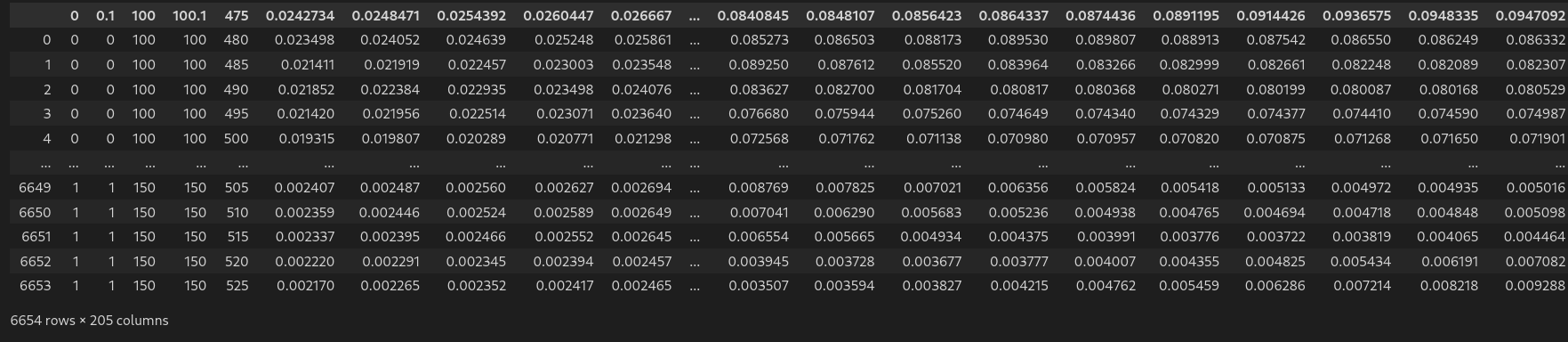
EXPLORING THE DATA: LOADING
Eosam 2024, 9-13 September 2024, Naples
# Loading data
filename = '../DL-Assisted-NHA-Inverse-Design-/Dataset 6655.csv'  # define filename
df = pd.read_csv(filename)  #load csv in dataframe
df  # display dataframe in notebook
EXPLORING THE DATA: FORMATTING
Eosam 2024, 9-13 September 2024, Naples
# Formatting the data
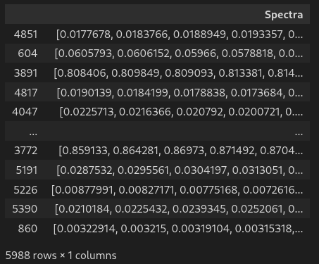
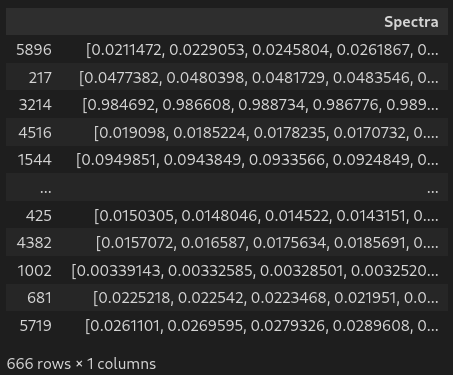
df['Spectra'] = df.values[:,5:][:,::-1].tolist() # gather 200 spectra column in one single list
df['Spectra'] = df['Spectra'].apply(np.array) # list to numpy array
df.drop(df.columns[5:-1], axis=1, inplace=True) # drop the gathered columns
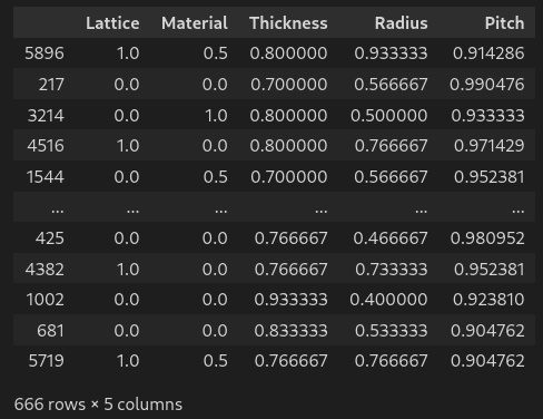
df.columns = ['Lattice','Material','Thickness','Radius','Pitch','Spectra'] # name all columns
df # display dataframe in notebook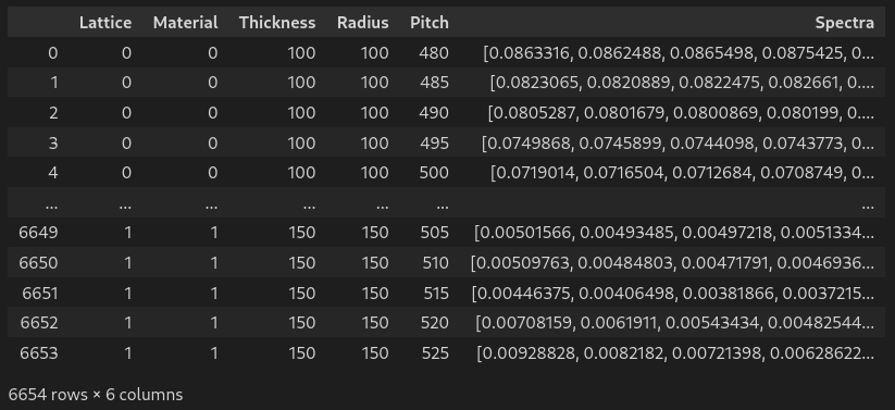
EXPLORING THE DATA: INSPECT
Eosam 2024, 9-13 September 2024, Naples
# Inspecting the data for unique values
df['Lattice'].sort_values().unique()
df['Material'].sort_values().unique()
df['Thickness'].sort_values().unique()
df['Radius'].sort_values().unique()
df['Pitch'].sort_values().unique()
# Unique values
array([0, 1]) # Lattice
array([0, 1, 2]) # Material
array([100, 105, 110, 115, 120, 125, 130, 135, 140, 145, 150]) # Thickness
array([ 50, 55, 60, 65, 70, 75, 80, 85, 90, 95, 100, 105, 110, 115, 120, 125, 130, 135, 140, 145, 150]) # Radius
array([475, 480, 485, 490, 495, 500, 505, 510, 515, 520, 525]) # PitchEXPLORING THE DATA: PLOT
Eosam 2024, 9-13 September 2024, Naples
# create vector for wavelengths
wl_min, wl_max, n_wl = 500.0, 1100.0, 200
wavelengths = np.linspace(wl_min,wl_max,n_wl)

# create figure canvas
fig,axs = plt.subplots(3,3,figsize = (15,10),sharex=True,sharey=False)

# pick 9 random samples
samples = np.random.randint(0,6553,9)

# loop over the plot 3x3 grid
for i in range(3):
    for j in range(3):

      	# create legend string depending on parameters
        legend_str = 'L=' + str(lattices[df['Lattice'].iloc[idx]]) + '\n' \
                     'M=' + str(materials[df['Material'].iloc[idx]]) + '\n' \
                     'R=' + str(df['Radius'].iloc[idx]) + ' (nm) \n' \
                     'T=' + str(df['Thickness'].iloc[idx]) + ' (nm) \n' \
                     'P=' + str(df['Pitch'].iloc[idx]) + ' (nm)'

        # plot data
        idx = samples[i*3+j]
        axs[i,j].plot(wavelengths,df['Spectra'].iloc[idx],label=legend_str)

        # plot x and y labels
        if i==2:
            axs[i,j].set_xlabel('Wavelength (nm)',fontsize= f_size)
        if j==0:
            axs[i,j].set_ylabel('Transmittance',fontsize= f_size)

        # tick label size
        axs[i,j].tick_params(labelsize=f_size-5)

        # display legend
        axs[i,j].legend(fontsize=f_size-8)

# set to tight plot layout
fig.set_tight_layout('tight')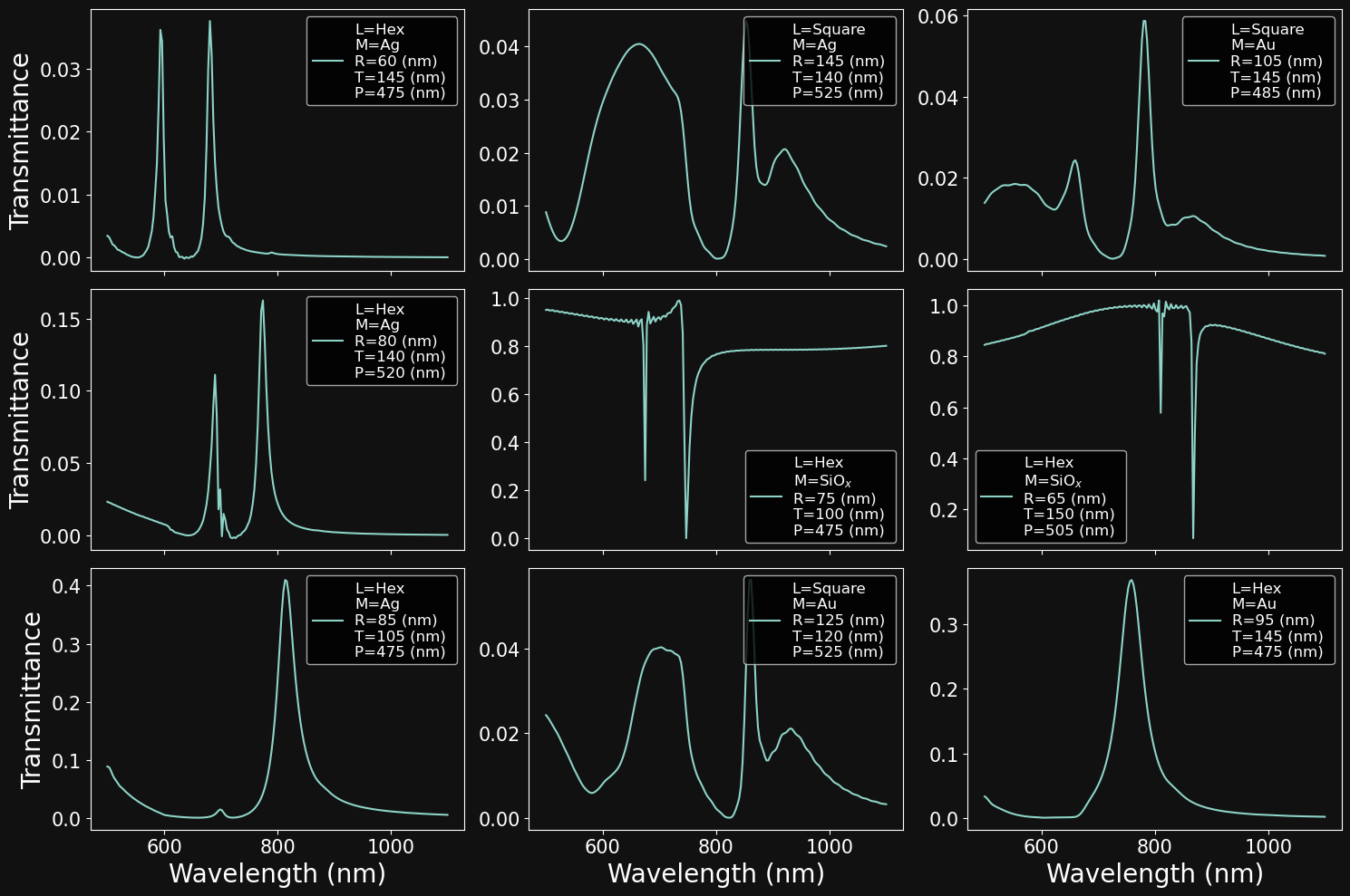
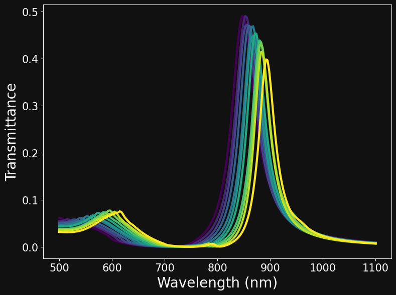
EXPLORING THE DATA: PARAMETER SWEEPS
Eosam 2024, 9-13 September 2024, Naples
# Select a set of parameters
L = 0 # hexagonal lattice
M = 0 # au material
R = 100 # radius
T = 125 # thickness
P = 500 # pitch
# Fix all parameters except pitch
df_pitch = df[(df.Lattice==L) & (df.Material==M) & (df.Radius==R) & (df.Thickness==T)]
df_pitch.sort_values(by=['Pitch'],inplace=True)
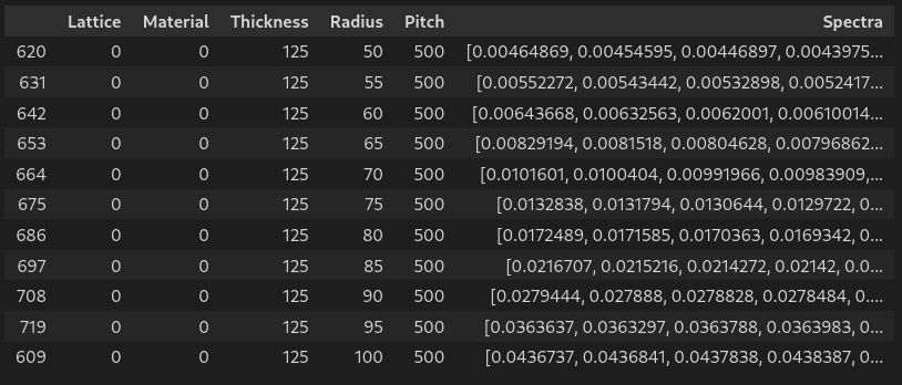
# Fig all parameters except radius
df_radius = df[(df.Lattice==L) & (df.Material==M) & (df.Pitch==P) & (df.Thickness==T)]
df_radius.sort_values(by=['Radius'],inplace=True)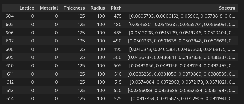
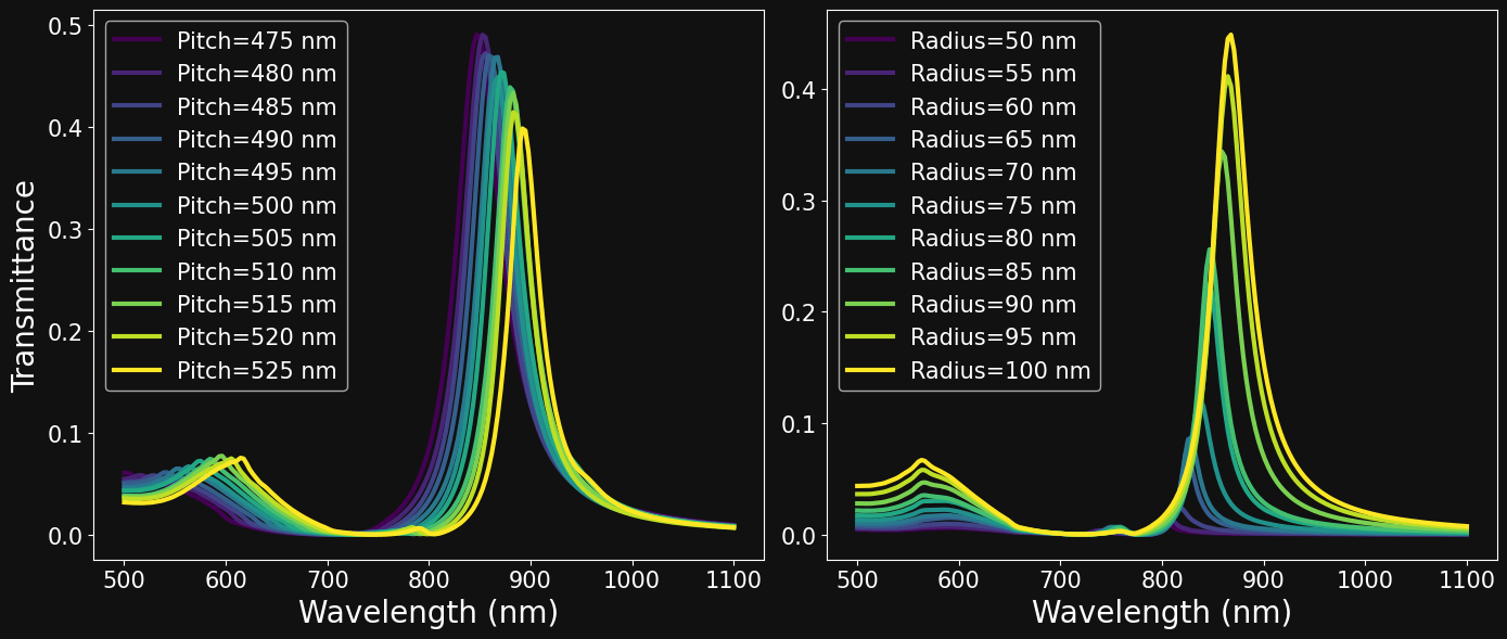
PITCH SWEEP
RADIUS SWEEP
TRAINING THE DIRECT NETWORK: LIBRARIES
Eosam 2024, 9-13 September 2024, Naples
Direct: \( g_{_{W}}:\mathbb{R}^{5} \to \mathbb{R}^{200} \)
# Importing auxiliary libraries
import numpy as np
import pandas as pd
import matplotlib.pyplot as plt
from sklearn.model_selection import train_test_split
from datetime import datetime

# import pytorch
import torch
import torch.nn as nn
from torch.utils.data import DataLoader


# import tensorboard for logging
from torch.utils.tensorboard import SummaryWriter

# importing local code
import sys
sys.path.append('../')
from datasets import SpectraDataset
from models import MLP, ResidualMLP
from loops import train,val
TRAINING THE DIRECT NETWORK: DATA PIPELINE
Eosam 2024, 9-13 September 2024, Naples
CLEAN AND PREPARE DATA
# filename
filename = './DL-Assisted-NHA-Inverse-Design-/Dataset 6655.csv'

# load in dataframe
df = pd.read_csv(filename)

# clean and rearrange data
df['Spectra'] = df.values[:,5:][:,::-1].tolist()
df['Spectra'] = df['Spectra'].apply(np.array)
df.drop(df.columns[5:-1], axis=1, inplace=True)
df.columns = ['Lattice','Material','Thickness','Radius','Pitch','Spectra']
CLEAN AND PREPARE DATA
TRAINING THE DIRECT NETWORK: DATA PIPELINE
Eosam 2024, 9-13 September 2024, Naples
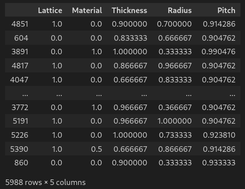
# select and normalize input features (X)
X_df = df[['Lattice','Material','Thickness','Radius','Pitch']]
X_df = X_df/X_df.max()

# select output labels (y)
y_df = df['Spectra']

# split in training and validation set
test_val_split = 0.1  # portion of data assigned to validation set
X_train, X_val, y_train, y_val = train_test_split(X_df, y_df, test_size=test_val_split, random_state=42)
SPLIT DATA IN TRAINING AND VALIDATION SET
\( X_{train} \)
\( X_{val} \)
\( y_{train} \)
\( y_{val} \)
TRAINING THE DIRECT NETWORK: DATA PIPELINE
Eosam 2024, 9-13 September 2024, Naples
# import libraries
import torch
import torch.utils.data as data
import numpy as np

class SpectraDataset(data.Dataset):
    """
    Custom dataset class for loading and processing spectral data.

    Args:
        X_df (pd.DataFrame): DataFrame containing the features.
        y_df (pd.DataFrame): DataFrame containing the labels.
    """

    def __init__(self, X_df, y_df):
        """
        Initializes the dataset with the provided features and labels.
        """

        # storing dataframes as features and labels
        self.X = X_df
        self.y = y_df

    def __len__(self):
        """
        Returns the length of the dataset (number of samples).
        """

        return len(self.X)

    def __getitem__(self, idx):
        """
        Retrieves a X and y pair for a given index.
        """

         # Extract features and labels from the data
        X = torch.tensor(self.X.iloc[idx].values.astype(np.float32))
        y = torch.tensor(self.y.iloc[idx].astype(np.float32))
        return X, y
CREATE AND INSTANTIATE DATASET
# instantiate training and validation dataset
training_dataset = SpectraDataset(X_train,y_train)
val_dataset = SpectraDataset(X_val,y_val)
TRAINING THE DIRECT NETWORK: DATA PIPELINE
Eosam 2024, 9-13 September 2024, Naples
CREATE DATALOADER
# batch size
batch_size = 64

# Create data loaders
train_dataloader = DataLoader(training_dataset, batch_size=batch_size, shuffle= True)
val_dataloader = DataLoader(val_dataset, batch_size=batch_size)

for X, y in val_dataloader:
    print(f"Shape of X [N, C]: {X.shape}")
    print(f"Shape of y: {y.shape} {y.dtype}")
    break
Shape of X [N, C]: torch.Size([64, 5])
Shape of y: torch.Size([64, 200]) torch.float32TRAINING THE DIRECT NETWORK: THE NEURAL NET
Eosam 2024, 9-13 September 2024, Naples
# pytorch building blocks
import torch.nn as nn

# Simple example of multilayer perceptron
class SimpleMLP(nn.Module):
    def __init__(self):
        super().__init__()

        # first layer
        self.linear1 = nn.Linear(5, 1000, bias=False)
        self.activation1 = nn.ReLU()

        # second layer
        self.linear2 = nn.Linear(1000, 1000, bias=False)
        self.activation2 = nn.ReLU()

        # third layer
        self.linear3 = nn.Linear(1000, 1000, bias=False)
        self.activation3 = nn.ReLU()

        # fourth layer
        self.linear4 = nn.Linear(1000, 1000, bias=False)
        self.activation4 = nn.ReLU()

        # fifth layer
        self.linear5 = nn.Linear(1000, 1000, bias=False)
        self.activation5 = nn.ReLU()

        # sixth layer
        self.linear6 = nn.Linear(1000, 200, bias=False)

    def forward(self, x):

        # forward pass of the nn
        x = self.linear1(x)
        x = self.activation1(x)
        x = self.linear2(x)
        x = self.activation2(x)
        x = self.linear3(x)
        x = self.activation3(x)
        x = self.linear4(x)
        x = self.activation4(x)
        x = self.linear4(x)
        x = self.activation4(x)
        x = self.linear5(x)
        x = self.activation5(x)
        x = self.linear6(x)

        return x
A VERY SIMPLE ARCHITECTURE
TRAINING THE DIRECT NETWORK: THE NEURAL NET
Eosam 2024, 9-13 September 2024, Naples
# 1pytorch building blocks
import torch.nn as nn

# a flexible, fully connected base block
class BaseBlock(nn.Module):
    def __init__(self, in_features, out_features, p=0.2, activation=nn.GELU()):
        super().__init__()
        self.linear = nn.Linear(in_features, out_features, bias=False)
        self.dropout = nn.Dropout(p=p)
        self.activation = activation

    def forward(self, x):
        x = self.linear(x)
        x = self.activation(x)
        x = self.dropout(x)
        return x

# a simple linear block for the direct regression problem
class LinearBlock(nn.Module):
    def __init__(self, in_features, out_features):
        super().__init__()
        self.linear = nn.Linear(in_features, out_features, bias=False)

    def forward(self, x):
        x = self.linear(x)
        return x
A FLEXIBLE ARCHITECTURE
# pytorch building blocks
import torch.nn as nn
from layers import BaseBlock, LinearBlock

# A flexible implementation of the multilayer perceptron
class FlexibleMLP(nn.Module):
    def __init__(
        self,
        hidden_layers=[5, 1000, 1000, 1000, 1000, 1000, 200],
        p=0.2,
        activation=nn.GELU(),
    ):
        super().__init__()

        self.layers = nn.ModuleList()
        for i in range(1, len(hidden_layers) - 1):
            self.layers.append(
                BaseBlock(
                    hidden_layers[i - 1], hidden_layers[i], p=p, activation=activation
                )
            )
        self.final_block = LinearBlock(hidden_layers[-2], hidden_layers[-1])

    def forward(self, x):
        for layer in self.layers:
            x = layer(x)
        x = self.final_block(x)
        return x
TRAINING THE DIRECT NETWORK: THE LOOP
Eosam 2024, 9-13 September 2024, Naples
# Get cpu or gpu device for training.
device = (
    "cuda"
    if torch.cuda.is_available()
    else "cpu"
)
print(f"Using {device} device")
CHOOSE DEVICE
# base learning rate
lr = 1.1e-4

# defining loss and optimizer
loss_fn = nn.MSELoss()
optimizer = torch.optim.Adam(model.parameters(),lr=lr)
LOSS AND LEARNING RATE
TRAINING THE DIRECT NETWORK: THE LOOP
Eosam 2024, 9-13 September 2024, Naples
# the training loop
def train(dataloader, model, loss_fn, optimizer, device):
    size = len(dataloader.dataset)
    model.train()
    for batch, (X, y) in enumerate(dataloader):
        X, y = X.to(device), y.to(device)

        # Compute prediction error
        pred = model(X)
        loss = loss_fn(pred, y)

        # Backpropagation
        loss.backward()
        optimizer.step()
        optimizer.zero_grad()

        if batch % 100 == 0:
            loss, current = loss.item(), (batch + 1) * len(X)
            print(f"Train loss: {loss:>7f}  [{current:>5d}/{size:>5d}]")

    return loss
TRAINING LOOP
- Training loop
- Dataset size
- Model in training mode (batchnorm, dropout, etc...)
- Loop over the dataset
- Move data to GPU
- Compute prediction and loss
- Compute gradients, update \( w^{i}_{jk}\), reset gradients
- Log loss at console
TRAINING THE DIRECT NETWORK: THE LOOP
Eosam 2024, 9-13 September 2024, Naples
# the validation loop
def val(dataloader, model, loss_fn, device):
    num_batches = len(dataloader)
    model.eval()
   val_loss = 0

    with torch.no_grad():
        for X, y in dataloader:
            X, y = X.to(device), y.to(device)
            pred = model(X)
            val_loss += loss_fn(pred, y).item()
    val_loss /= num_batches
    print("\n")
    print(f"Validation loss: {val_loss:>8f} \n")

    return val_loss
VALIDATION LOOP
- Validation loop
- Number of batches contained in the dataset
- Model in eval mode (no dropout, batchnorm, etc...)
- Loop over the dataset
- Move data to GPU
- Compute prediction and accumulate loss
- Log average loss at console
- Reset validation loss
- Turn off gradients
TRAINING THE DIRECT NETWORK: THE LOOP
Eosam 2024, 9-13 September 2024, Naples
# create timestamp
now = datetime.now()  # current date and time
date_time = now.strftime("%d%m%y_%H%M%S")

# create summary writer for tensorboard
writer_path = '../tb_logs/' + date_time + '/'
writer = SummaryWriter(writer_path)

# loop over epochs
epochs = 2500
epoch_threshold = 500
save_checkpoint = './best_model_' + date_time + '.ckpt'
best_loss = 1.0
for epoch in range(epochs):

    # log epoch to console
    print(f"Epoch {epoch+1}\n-------------------------------")

    # performe training and validation loops
    train_loss = train(train_dataloader, model, loss_fn, optimizer, device)
    val_loss = val(val_dataloader, model, loss_fn, device)

    # log training and validation loss to console
    writer.add_scalar("Loss/train", train_loss, epoch)
    writer.add_scalar("Loss/val", val_loss, epoch)

    # save checkpoint
    if (val_loss < best_loss) and (epoch>epoch_threshold):

        # save checkpoint
        model.train()
        torch.save(model.state_dict(), save_checkpoint)
        best_loss = val_loss

# close connection to tensorboard
writer.flush()
writer.close()

# finished
print("Done!")
OPTIMIZATION LOOP
- Create timestamp for logging
- Setup Tensorboard logging
- Loop over epochs (1 epoch = whole dataset pass)
- Log to Tensorboard
- Close connection to Tensorboard
- Log epoch to console
- Perform training and validation loops
- Save best checkpoint
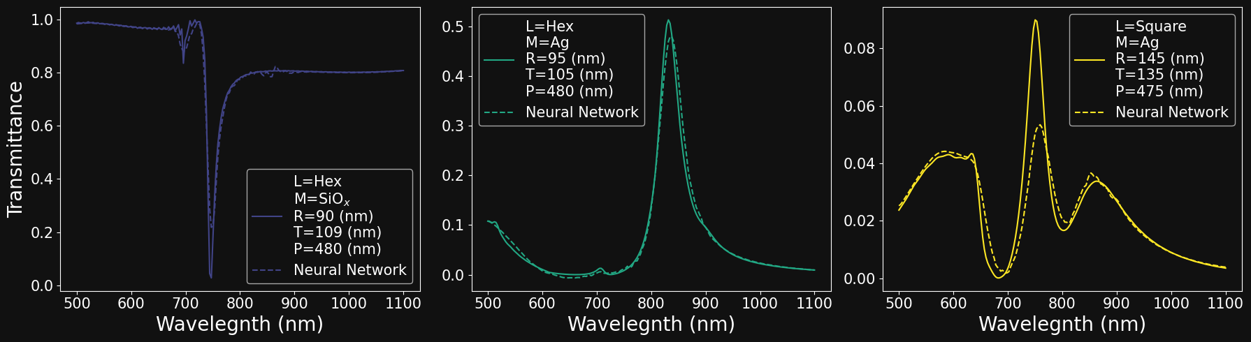
MODEL INFERENCE
Eosam 2024, 9-13 September 2024, Naples
# Instantiate inference model and set to evaluation mode
model_inference = FlexibleMLP(hidden_layers=hidden_layers, activation=nn.GELU(), p=0.1).to(
    device)
model_inference.load_state_dict(torch.load(save_checkpoint,weights_only=True))
model_inference.eval()

# compute inference on all validation samples
X_inference = torch.tensor(X_val.to_numpy().astype(np.float32)).to(device)
y_inference = model_inference(X_inference)
y_true = torch.tensor(np.stack(y_val.to_numpy()).astype(np.float32)).to(device)

# compute normalized loss for each sample in the validation dataset
loss_fn_inference = nn.MSELoss(reduction='none')
with torch.no_grad():
    loss_inference = loss_fn_inference(y_inference,y_true).sum(axis=-1)
norm_mse_discrepancy = loss_inference/((y_true**2).sum(axis=-1))
k_best = torch.argsort(norm_mse_discrepancy)- Load checkpoint
- Inference on all validation data
- Loss for every validation sample
SOLVING THE INVERSE PROBLEM
Eosam 2024, 9-13 September 2024, Naples
# 1pytorch building blocks
import torch.nn as nn

# a flexible, fully connected, multi headed network
class FlexibleInverseMLP(nn.Module):
    def __init__(
        self,
        hidden_layers=[200, 1000, 1000, 1000, 1000, 1000, 2, 3, 3],
        p=0.2,
        activation=nn.GELU(),
    ):
        super().__init__()

        self.layers = nn.ModuleList()
        for i in range(1, len(hidden_layers) - 3):
            self.layers.append(
                BaseBlock(
                    hidden_layers[i - 1], hidden_layers[i], p=p, activation=activation
                )
            )

        # define 2 classification heads and 1 regression head
        self.lattice_head = LinearBlock(hidden_layers[-4], hidden_layers[-3])
        self.material_head = LinearBlock(hidden_layers[-4], hidden_layers[-2])
        self.geometry_head = LinearBlock(hidden_layers[-4], hidden_layers[-1])

    def forward(self, x):

        # common path
        for layer in self.layers:
            x = layer(x)

        # three heads
        x_lattice = self.lattice_head(x)
        x_material = self.material_head(x)
        x_geometry = self.geometry_head(x)

        return x_lattice,x_material,x_geometry
A MULTI-HEADED FLEXIBLE ARCHITECTURE
TRAINING THE INVERSE NETWORK: THE LOOP
Eosam 2024, 9-13 September 2024, Naples
# the inverse training loop
def train_inverse(dataloader, model, loss_reg, loss_ce, optimizer, device):
    size = len(dataloader.dataset)
    model.train()
    for batch, (X, y) in enumerate(dataloader):
        X, y = X.to(device), y.to(device)

        # Compute prediction error
        pred_l, pred_m, pred_g = model(X)
        true_l = y[:,0].type(torch.LongTensor).to(device)
        true_m = y[:,1].type(torch.LongTensor).to(device)
        true_g = y[:,2:].to(device)

        loss = loss_ce(pred_l, true_l) + loss_ce(pred_m, true_m) + 5.0*loss_reg(pred_g, true_g)

        # Backpropagation
        loss.backward()
        optimizer.step()
        optimizer.zero_grad()

        if batch % 20 == 0:
            loss, current = loss.item(), (batch + 1) * len(X)
            print(f"Train loss: {loss:>7f}  [{current:>5d}/{size:>5d}]")

    return loss
TRAINING LOOP
- Training loop
- Dataset size
- Model in training mode (batchnorm, dropout, etc...)
- Loop over the dataset
- Move data to GPU
- Compute prediction and loss
- Compute gradients, update \( w^{i}_{jk}\), reset gradients
- Log loss at console
TRAINING THE INVERSE NETWORK: THE LOOP
Eosam 2024, 9-13 September 2024, Naples
# the inverse validation loop
def val_inverse(dataloader, model, loss_reg, loss_ce, device):
    num_batches = len(dataloader)
    model.eval()
    val_loss = 0

    with torch.no_grad():
        for X, y in dataloader:
            X, y = X.to(device), y.to(device)
            pred_l, pred_m, pred_g = model(X)
            true_l = y[:,0].type(torch.LongTensor).to(device)
            true_m = y[:,1].type(torch.LongTensor).to(device)
            true_g = y[:,2:].to(device)
            loss = loss_ce(pred_l, true_l) + loss_ce(pred_m, true_m) + loss_reg(pred_g, true_g)
            val_loss += loss.item()

    val_loss /= num_batches
    print("\n")
    print(f"Validation loss: {val_loss:>8f} \n")

    return val_loss
VALIDATION LOOP
- Validation loop
- Number of batches contained in the dataset
- Model in eval mode (no dropout, batchnorm, etc...)
- Loop over the dataset
- Move data to GPU
- Compute prediction and accumulate loss
- Log average loss at console
- Reset validation loss
- Turn off gradients
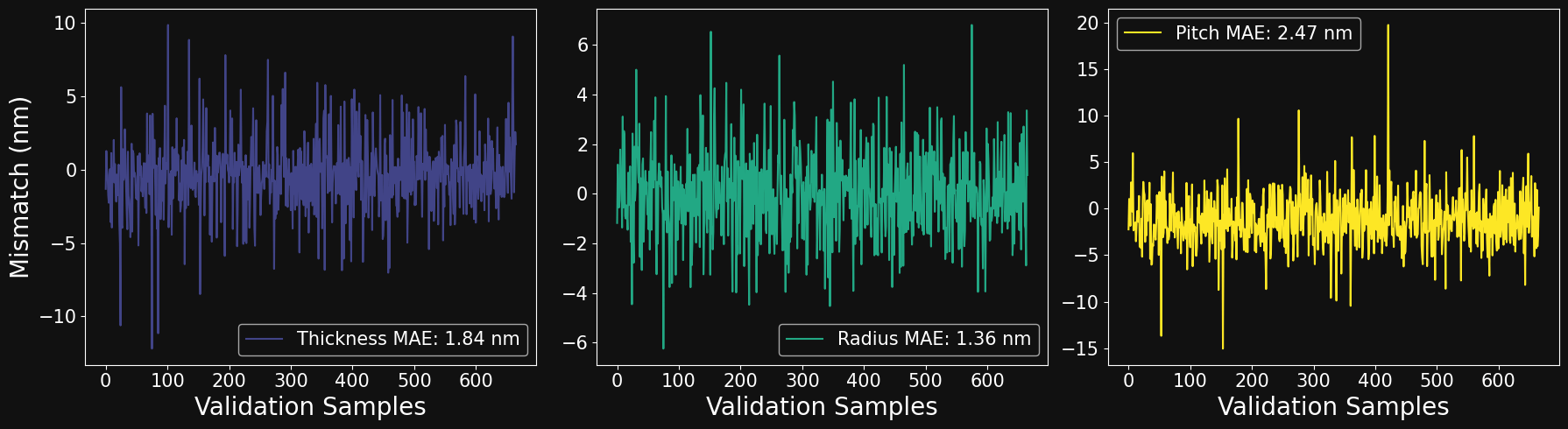
INVERSE MODEL INFERENCE
Eosam 2024, 9-13 September 2024, Naples
# Instantiate inference model and set to evaluation mode
model_inference = FlexibleInverseMLP(hidden_layers=hidden_layers, activation=nn.GELU(), p=0.1).to(
    device)
model_inference.load_state_dict(torch.load(save_checkpoint,weights_only=True))
model_inference.eval()

# compute inference on all validation samples
X_inference = torch.tensor(np.stack(X_val.to_numpy()).astype(np.float32)).to(device)
y_inf_lattice, y_inf_material, y_inf_geometry = model_inference(X_inference)
y_true = torch.tensor(y_val.to_numpy().astype(np.float32)).to(device)

# formatting true values for each classification and regression task
y_true_lattice = y_true[:, 0].type(torch.LongTensor).detach().cpu()
y_true_material = y_true[:, 1].type(torch.LongTensor).detach().cpu()
y_true_geometry = (
    torch.stack((y_true[:, 2] * t_max, y_true[:, 3] * r_max, y_true[:, 4] * p_max))
    .T.detach()
    .cpu()
)

# formatting predicted values for each classification and regression task
y_pred_lattice = (
    torch.argmax(torch.nn.functional.softmax(y_inf_lattice, dim=-1), dim=-1)
    .detach()
    .cpu()
)
y_pred_material = (
    torch.argmax(torch.nn.functional.softmax(y_inf_material, dim=-1), dim=-1)
    .detach()
    .cpu()
)
y_pred_geometry = (
    torch.stack(
        (
            y_inf_geometry[:, 0] * t_max,
            y_inf_geometry[:, 1] * r_max,
            y_inf_geometry[:, 2] * p_max,
        )
    )
    .T.detach()
    .cpu()
)- Load checkpoint
- Inference on all validation data
- Format the data to visualize inference results
HAPPY TRAINING!!!
Eosam2024Tutorial
By Giovanni Pellegrini


