Multi-resolution Scarlet

Rémy Joseph, Peter Melchior, Fred Moolekamp, JiaXuan Li

Modelling astro images for
Deblending
Galaxy light profile
Telescope refraction (convolution)
Instrument acquisition (pixelation)
Instrumental noise
(PM)_{[x,y]}+N_{[x,y]}
(R*H*M)_{[x,y]}
H*M
M

PSF:
R*H
In practice
I_{[x,y]} = (P\sum_i M_i)_{[x,y]}+N_{[x,y]}
Scarlet:
Multi-band deblending
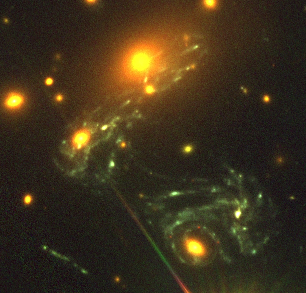
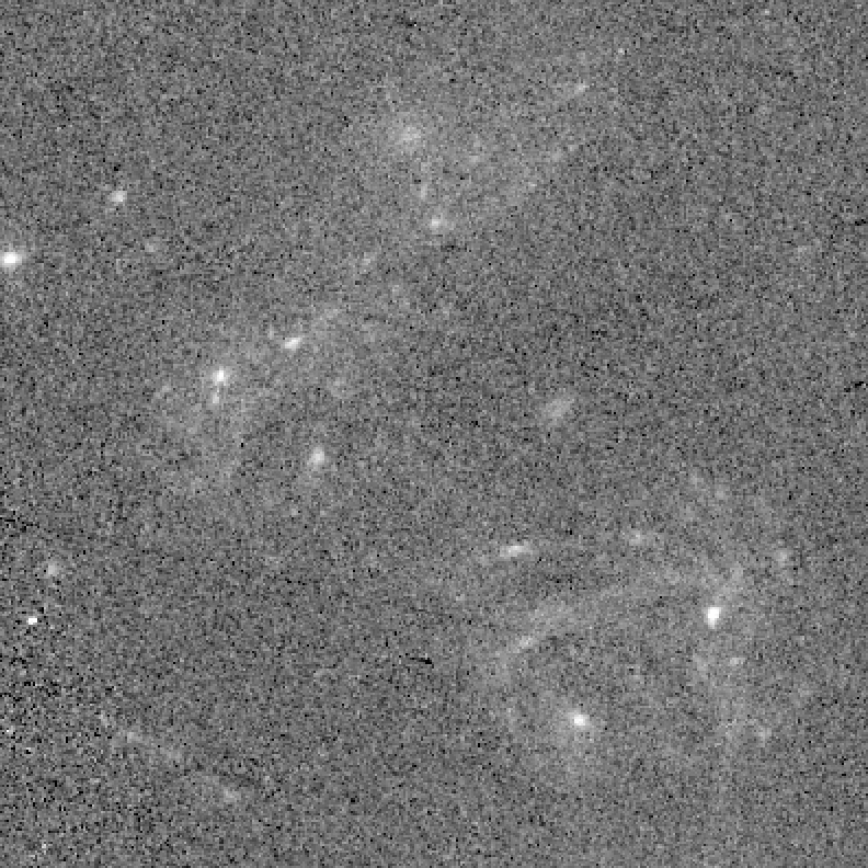
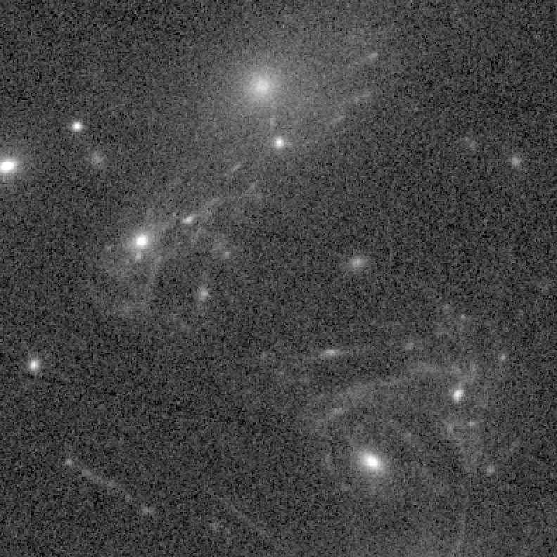
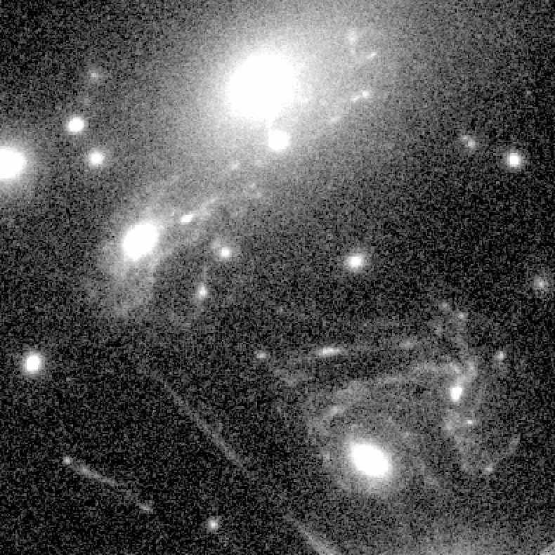
F435w
F606w
F814w
NASA/ESA: Hubble Frontier Fields, MACSJ 1149, Lotz et al. (2016)
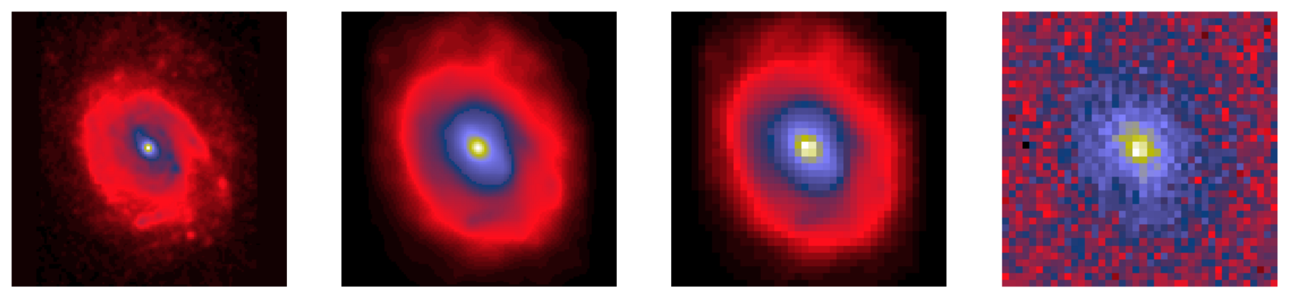
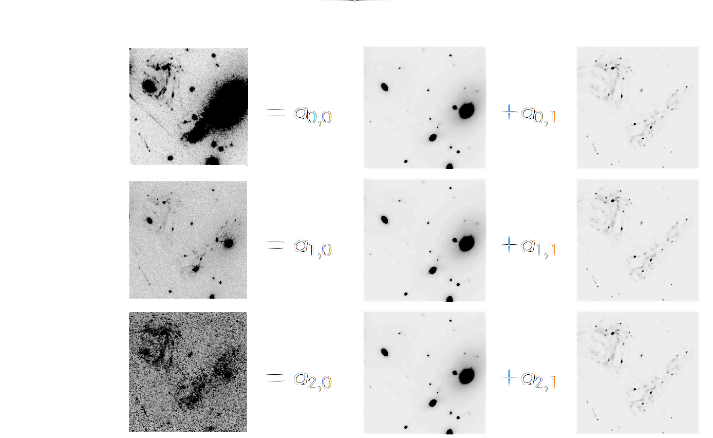
- RGB images are collections of band in different filters
SCARLET
- Colour-based: each band is a linear combination of monochromatic components
F435w: \(I_2\)
F606w: \(I_1\)
F814w: \(I_0\)
$$I_j = H_j * \sum_i a_{j,i}m_i + N_j$$
$$m_0$$
$$m_1$$
$$I$$
pixels
wavelength
pixels
pixels
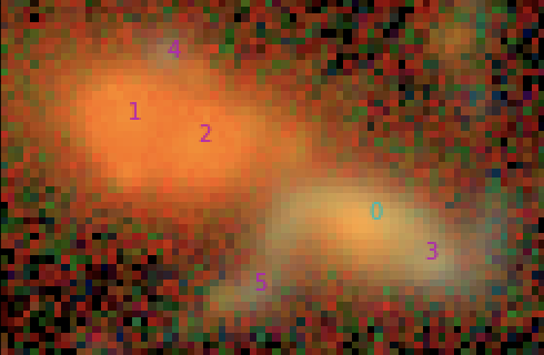
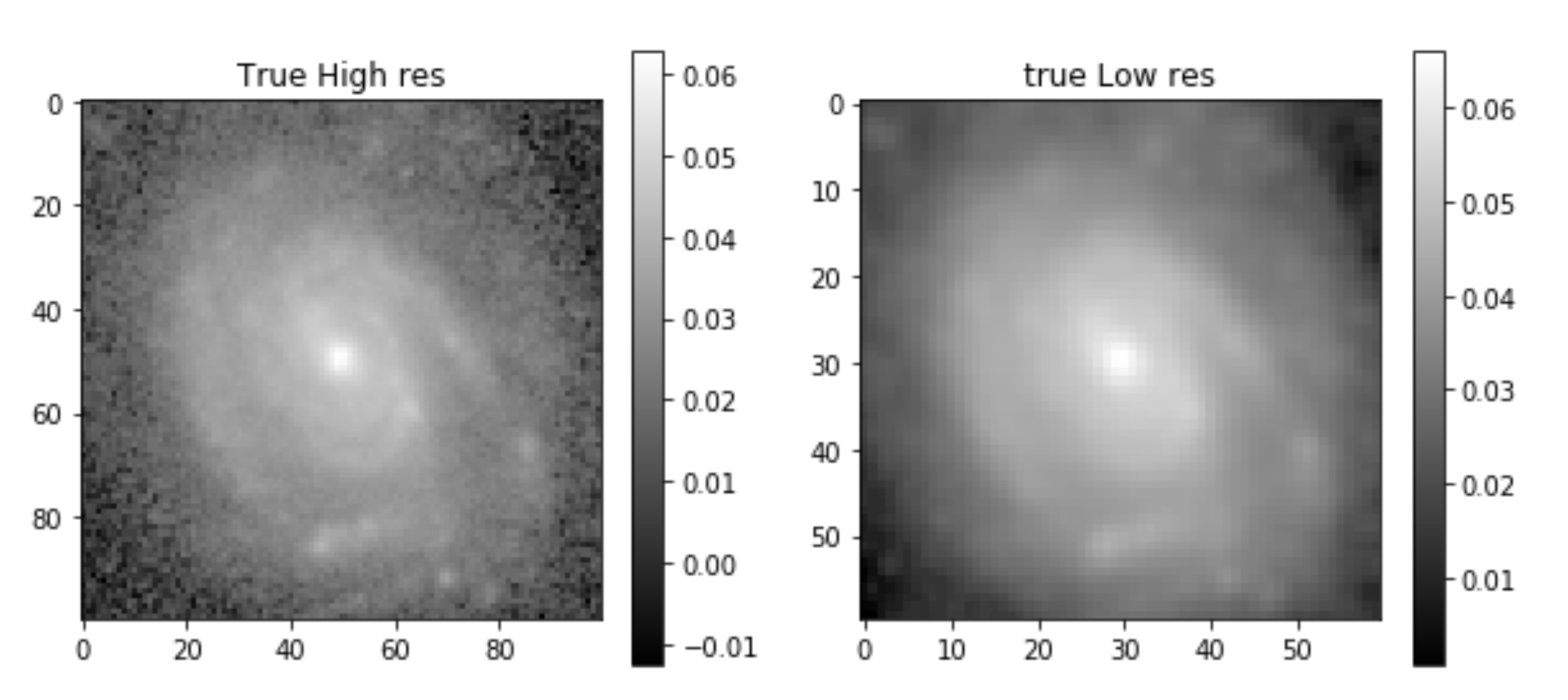
Multi-resolution deblending: Same idea, different resolutions
HST cosmos, F814w
HSC DR2, grizy
\(Y_1\):
\(Y_2\):
pixels
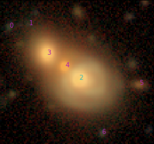
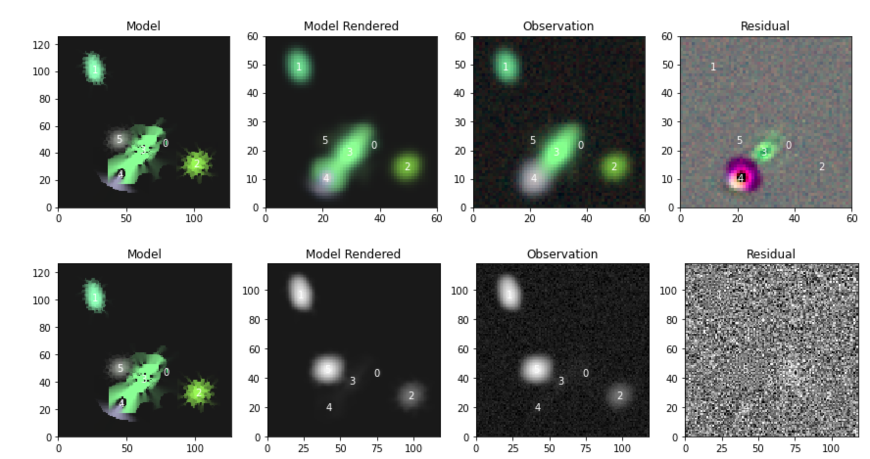
Scarlet model
1
2
4
3
5
6
Interpolation at different resolution
General formula for interpolation
\(f(x, y) = \sum_{x_k, y_j} f(x_k, y_j) K(x-x_k, y-y_j)\)
Interpolation kernel
Known samples
Samples at desired position (x, y)
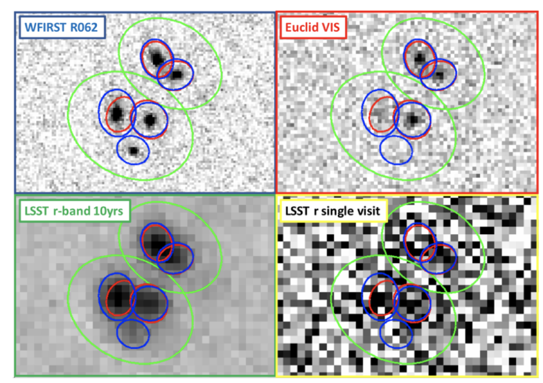
Euclid-like
HST-like
?
Euclid-like
HST-like
Interpolation at different resolution
Astronomical images have different samplings & different PSFs!!
\(f_1(x, y) = (f*h_1)(x_{}, y)\)
\(f_2(X, Y) = (f*h_2)(X, Y)\)
Shannon-Whittaker interpolation
\((f*p)(t_m) = (F*S)*(P*S)\) = F*P*S
\(f(t_m) = h\sum_{t_k}f(t_k)sinc(\frac{t_k-t_m}{h}) = F*S\)
Interpolation and convolution
\( (f*p)(x_{mx},y_{my}) = h^2 \sum_{x_{kx},x_{ky}} f(x_{kx}, y_{ky})\sum_{x_{lx}, y_{ly}}p(x_{lx},y_{ly})sinc(\frac{x_{mx}-x_{kx}-x_{lx}}{h})sinc(\frac{y_{my}-y_{ky}-x_{ly}}{h})\)
\(I_2(x_{i2},y_{j2}) = (f*p_2) (x_{i2},y_{j2}) = \\ h^2 \sum_{y_{j1}} \sum_{x_{k1}}\sum_{x_{i1}} F(x_{i1}, y_{j1}) sinc(\frac{x_{i2}-x_{i1}-x_{k1}}{h} )\sum_{y_{l1}} P_d(x_{k1}, y_{l1})sinc(\frac{y_{j2}-y_{j1}-y_{l1}}{h}) \)
The problem of speed
\(f(X, Y) = \sum_{x_k, y_j} f(x_k, y_j) p(X-x_k, Y-y_j)\)
\((X,Y)\) and \((x_k, y_j)\) are not on the same grid.
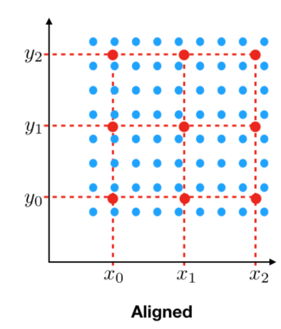
The problem of speed
\(f_2(X, Y) = \sum_{x_k, y_j} f_1(x_k, y_j) p(X-x_k, Y-y_j)\)
As many operations as there are distances between red and blue points, i.e. \(M^2N^2\)
M
N
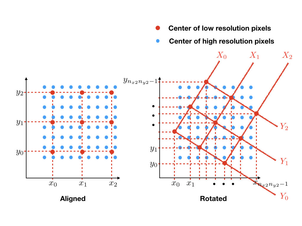
The problem of speed
\(f_2(X, Y) = \sum_{x_k, y_j} f_1(x_k, y_j) P(\frac{X}{h}-x_k, \frac{Y}{h}-y_j)\)
\(X = hX_1cos\theta + hY_1sin\theta\)
\(Y = -hX_1sin\theta + hY_1cos\theta\)
Shifts along two directions
Reformulate to share the distance calculations along directions of constant coordinates:
\(f_2(X, Y) = \sum_{x_k, y_j} f_1(x_k-X_1cos\theta, y_j+X_1sin\theta) \times P(-Y_1sin\theta-x_k, -Y_1cos\theta-y_j)\)
The problem of speed
\(f_2(X, Y) = \sum_{x_k, y_j} f_1(x_k-X_1cos\theta, y_j+X_1sin\theta) \times P(-Y_1sin\theta-x_k, -Y_1cos\theta-y_j)\)
- Shifts along \(2\times M\) directions instead of \(M^2\)
- Multiplcation of two matrices : \(N^2M \times MN^2\) instead of \(N^2\times N^2M^2\)
- Orders of magnitude faster than computing and multiplying by the \(P(X-x_k, Y-y_j)\) kernel
Interpolation at different resolution
Euclid-like
HST-like
Resampling and difference convolution can be done as one operation:
\(f_2(X, Y) = \sum_{x_k, y_j} f_1(x_k, y_j) H(X-x_k, Y-y_j)\)
Interpolation with difference kernel as the interpolation kernel. (Demo-ish in back up slide)
\(P(x,y) = \mathcal{F}^{-1}(\frac{\tilde{h_2}}{\tilde{h_1}})(-x,-y)\)
Comparison with galsim:
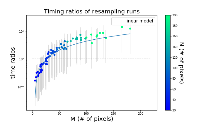
t = 0.046M - 0.2
Galsim interpolation scheme:
Interpolation kernel is reduced to a quintic kernel of size kxk = 6x6. requires s=4-fold padding.
Complexities:
- Galsim: $$O(N^2(k^2+s^2log(sN))+M^2(3+log(M)))$$
- Scarlet: $$O(N^2(M+1)(log(N)+M))$$
Comparison with galsim:
Reconstructions
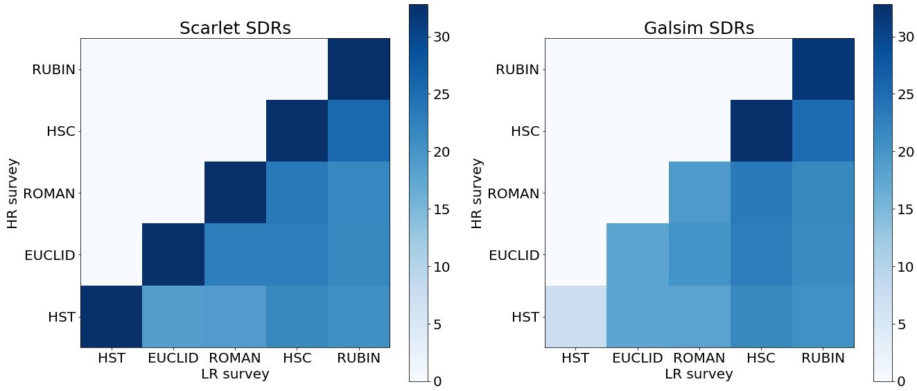
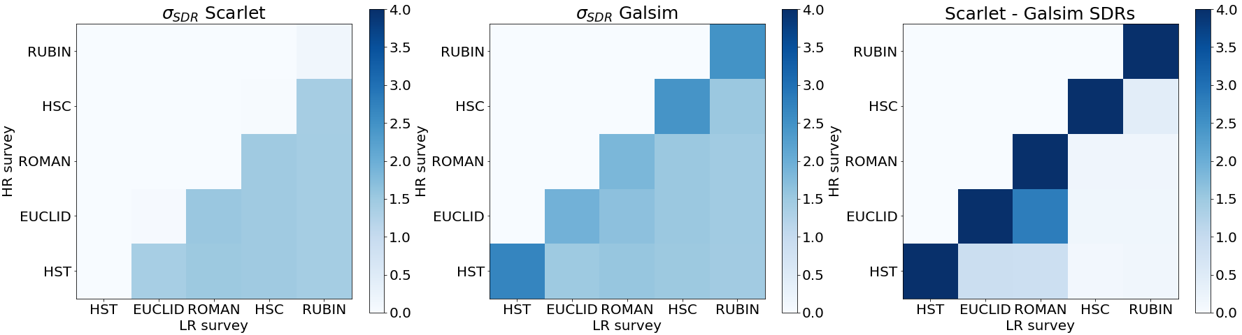
Comparison of source distortion ratios between Galsim and Scarlet interpolations
$$SDR(\tilde{X}) = 10\log_{10}(\frac{||X_{true}||}{||\tilde{X} - X_{true}||} )$$
Gains from Multi-resolution
Comparison of SDR in deblending of Euclid, Rubin and Euclid+Rubin images.
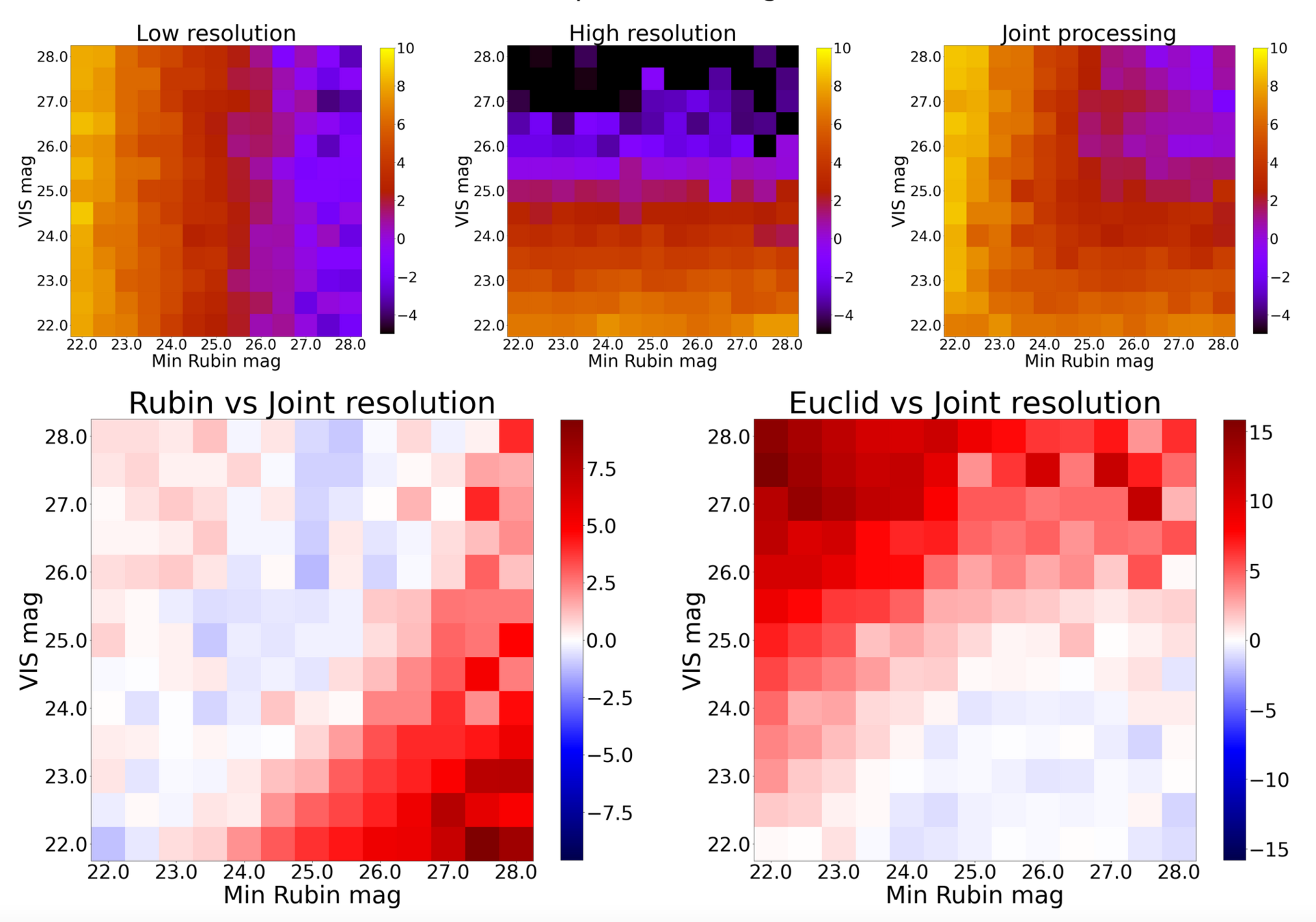
Gains from Multi-resolution
Comparison of SDR in deblending of Euclid, Rubin and Euclid+Rubin images.
The issue: initialisation
The problem of detection
Credit: Ranga Ram Chary
The problem of detection
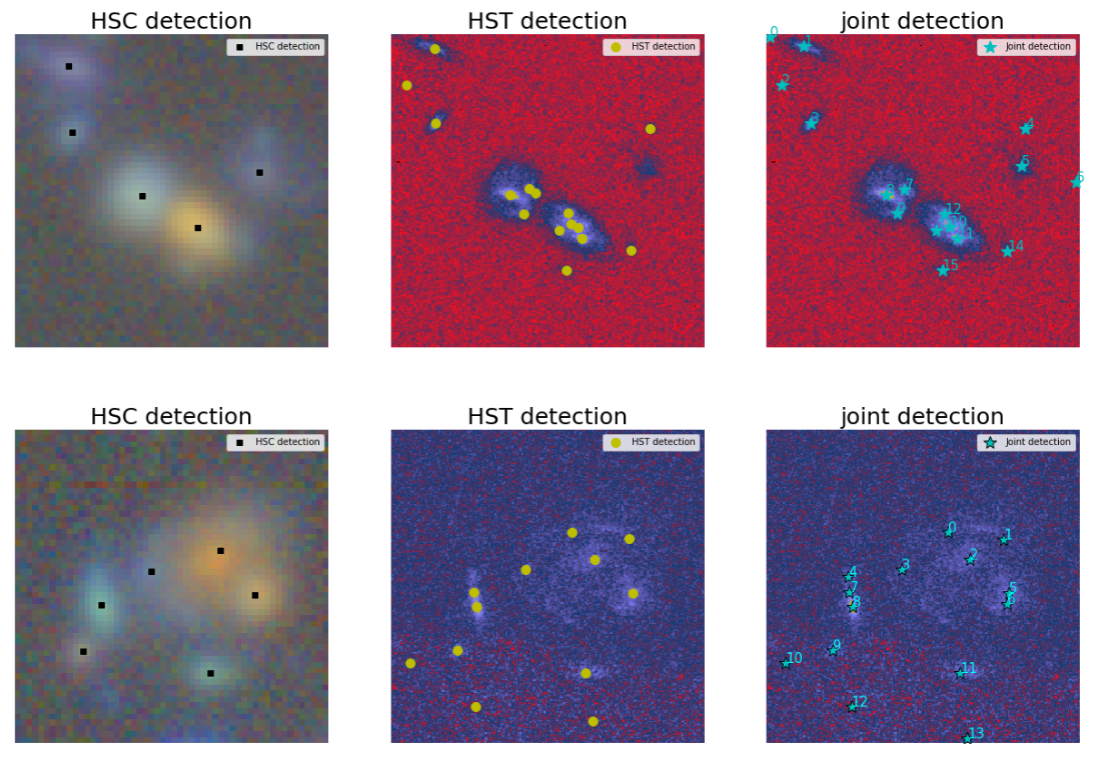
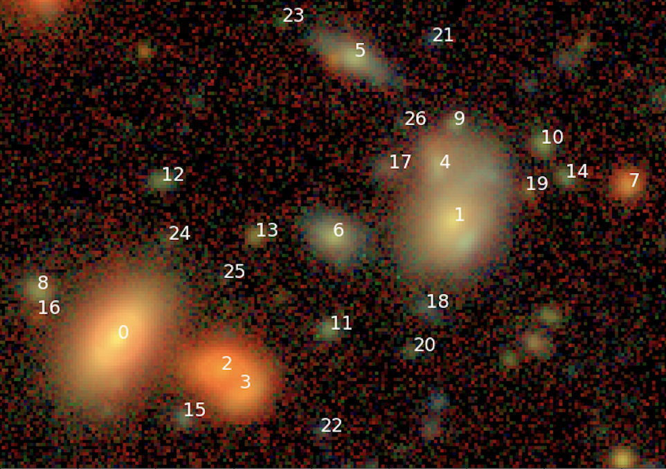
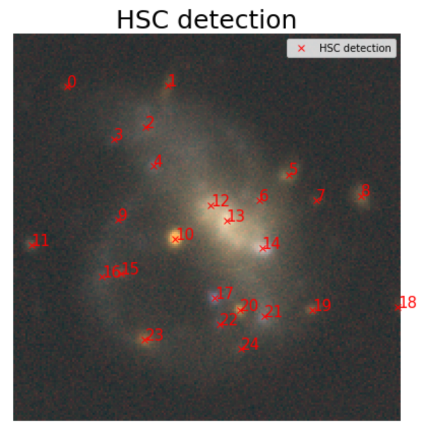
Multi-band detection with SEP:
- Build a coadd of all bands
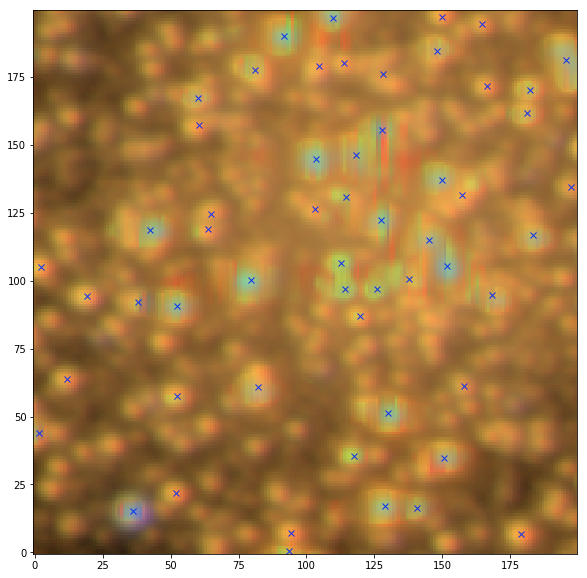
- Apply Starlet filter to select High frequencies
- Run sep on the filtered Coadds
Multi-resolution detection
- Interpolation of low resolution image to high resolution
- Coadd interpolated images and High resolution bands
- Idem as before
Side note:
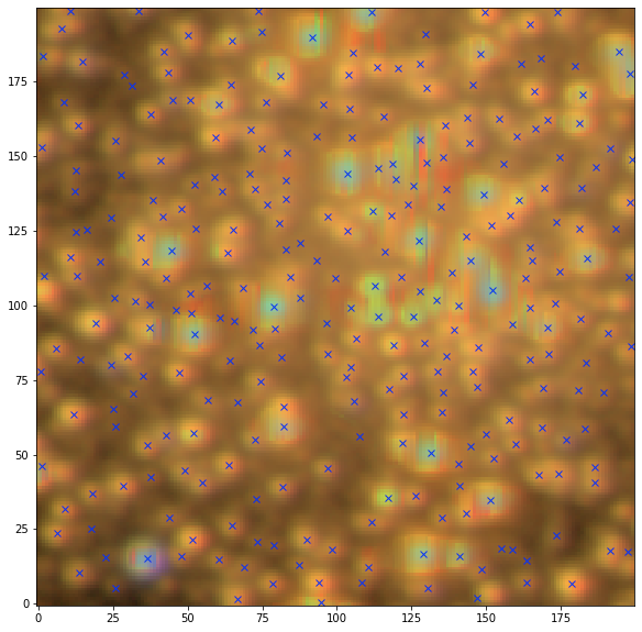
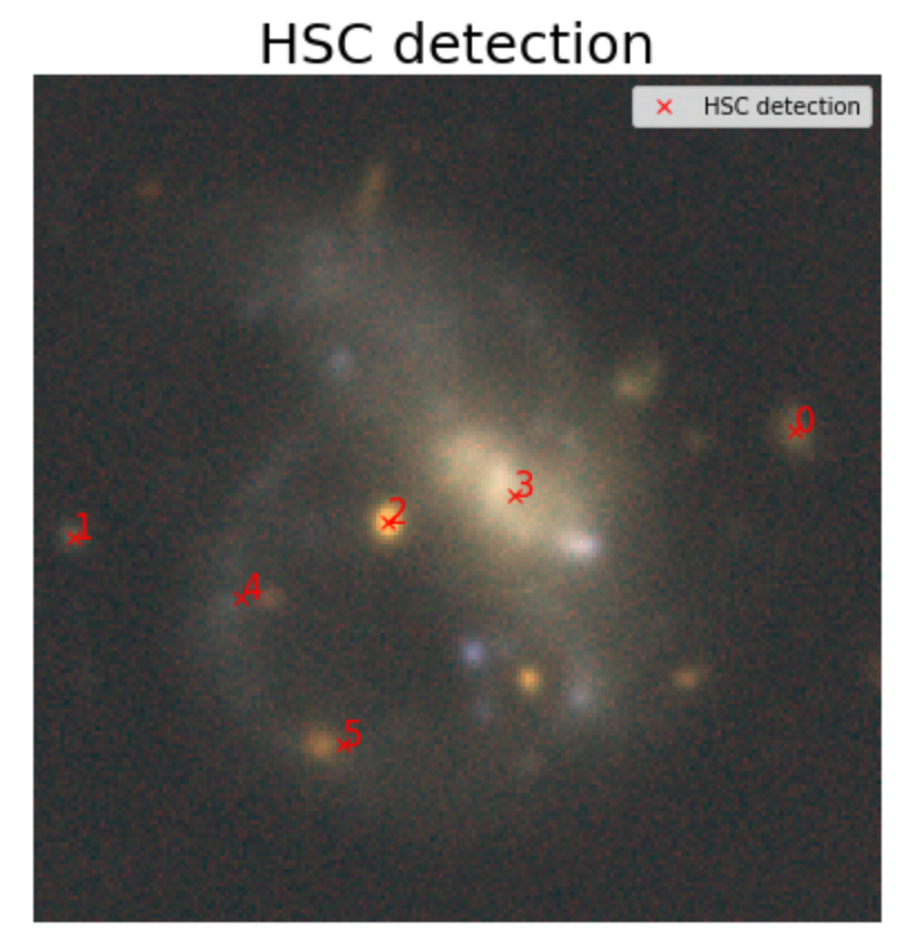
SEP detection
SEP + Starlet detection
Credit: Fred Moolekamp
Astrometry
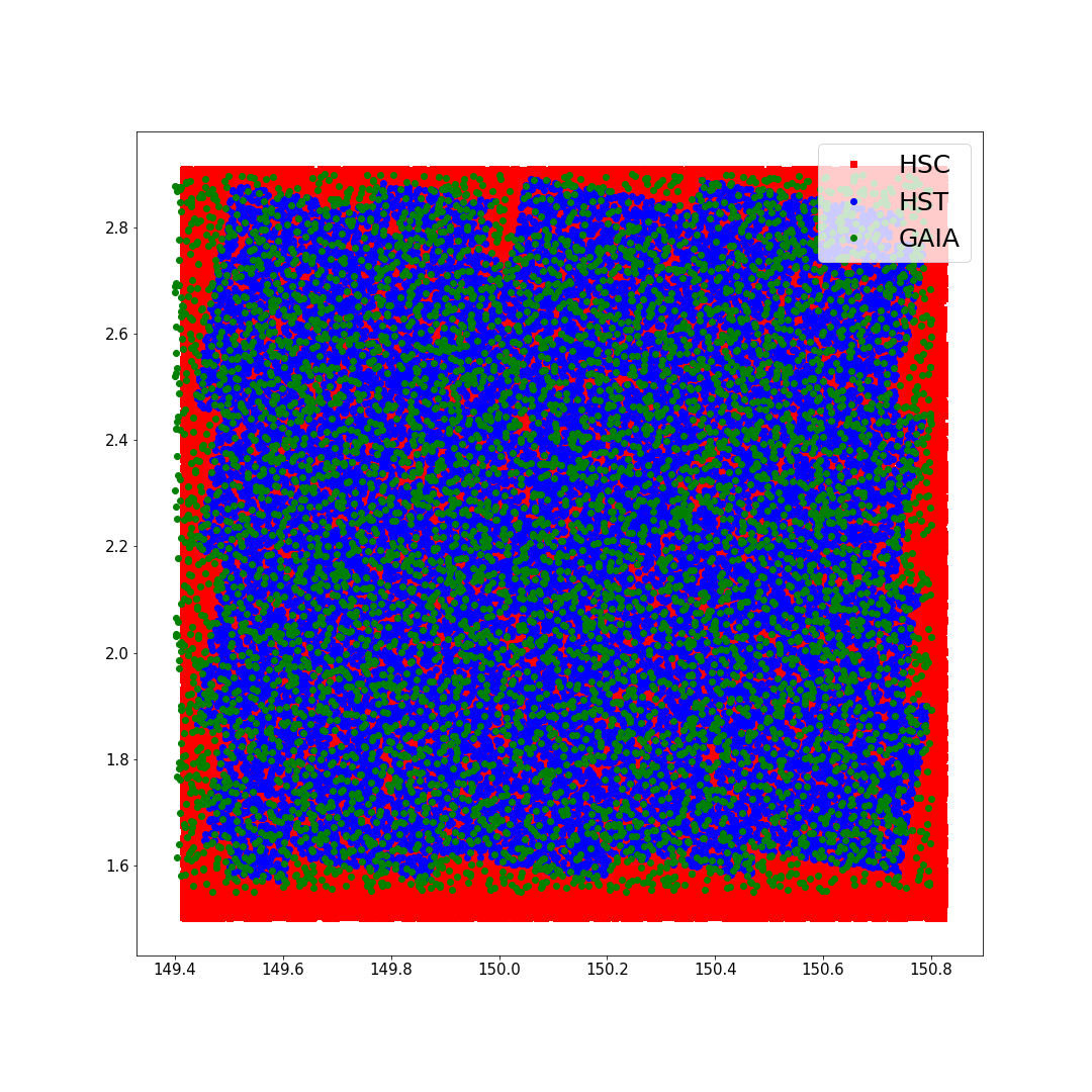
COSMOS Fields
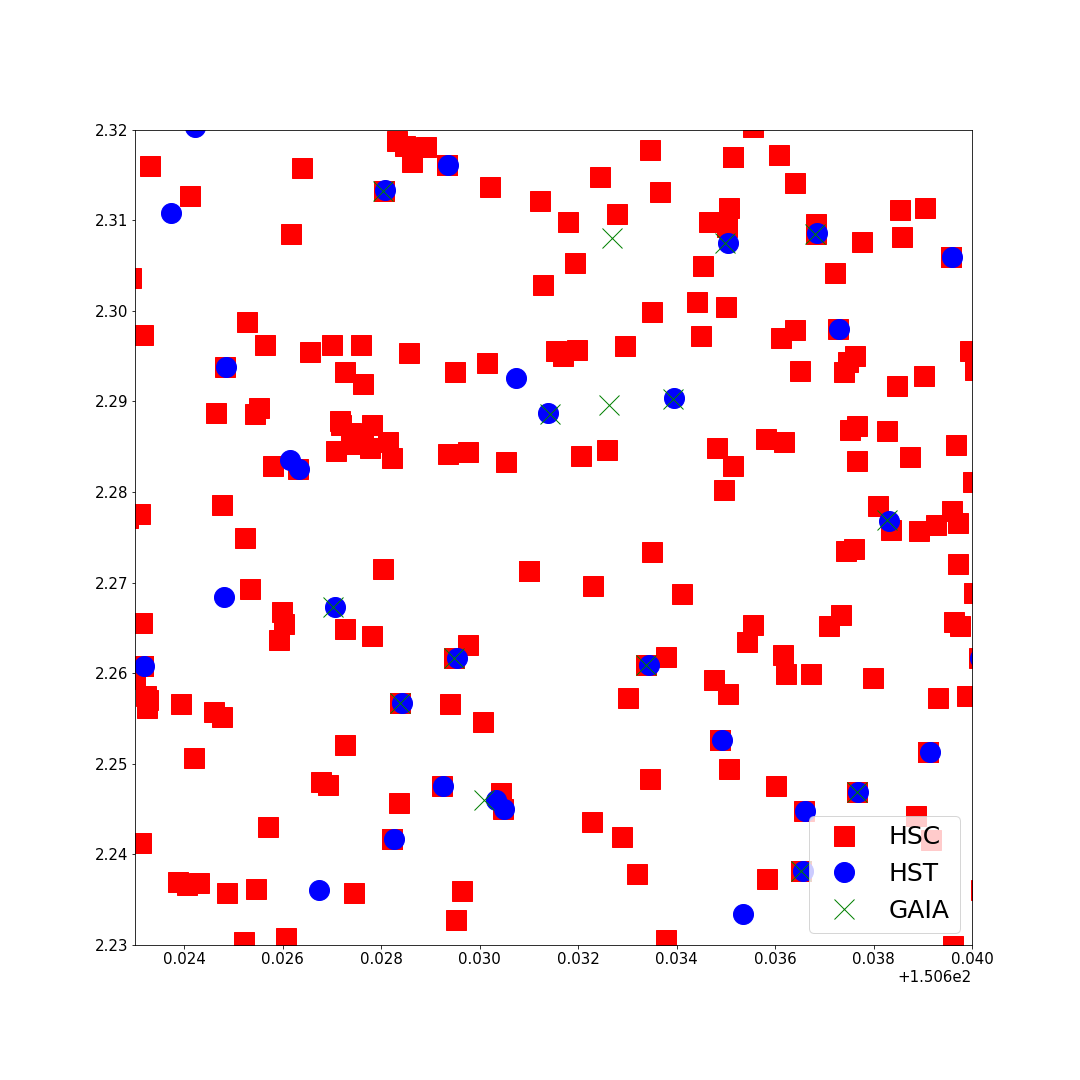
Matching observations, requires matching object positions
Astrometry
HST - HSC positions
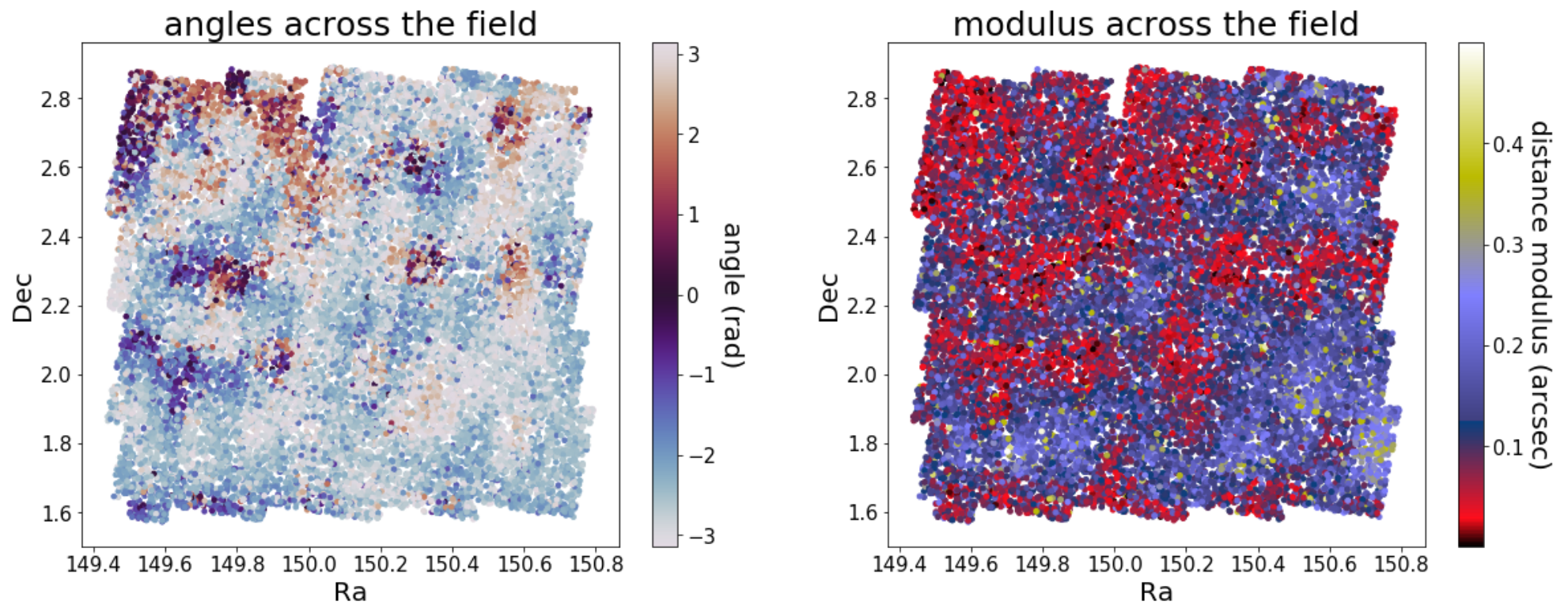
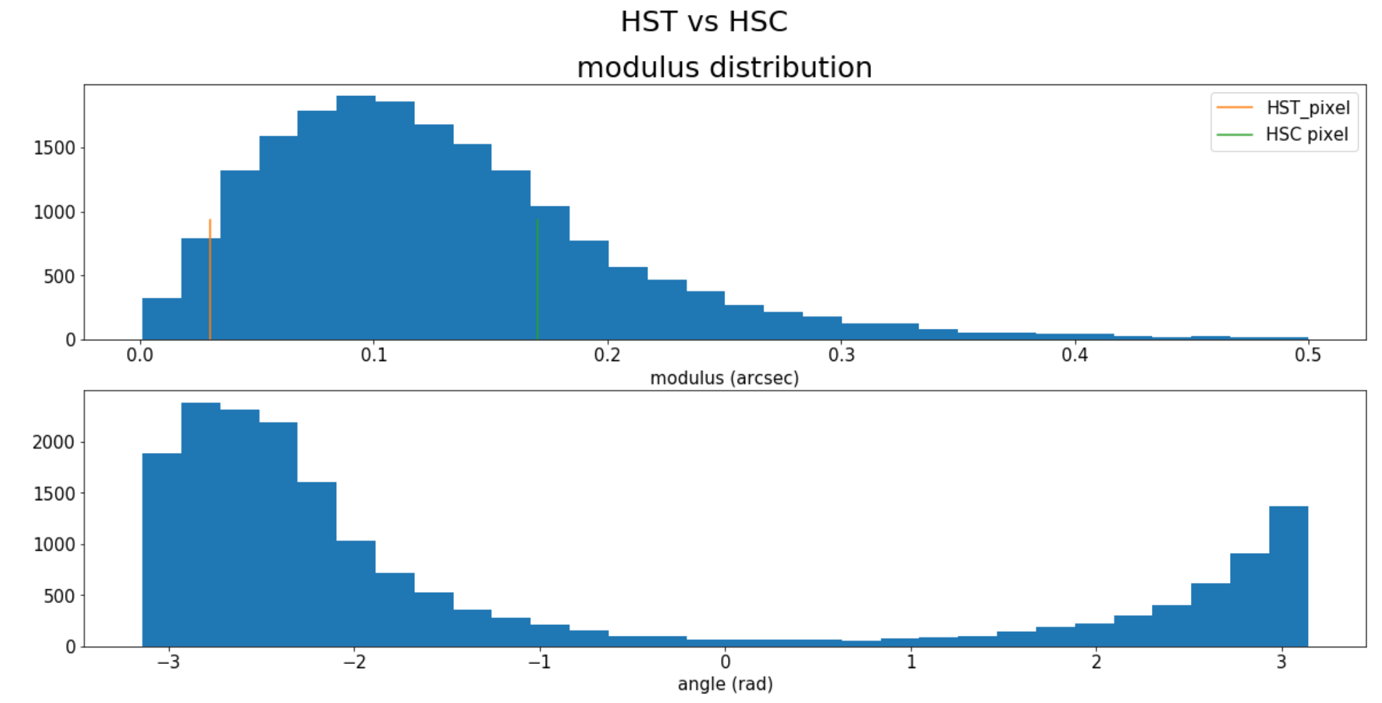
HSC s18 dud catalog
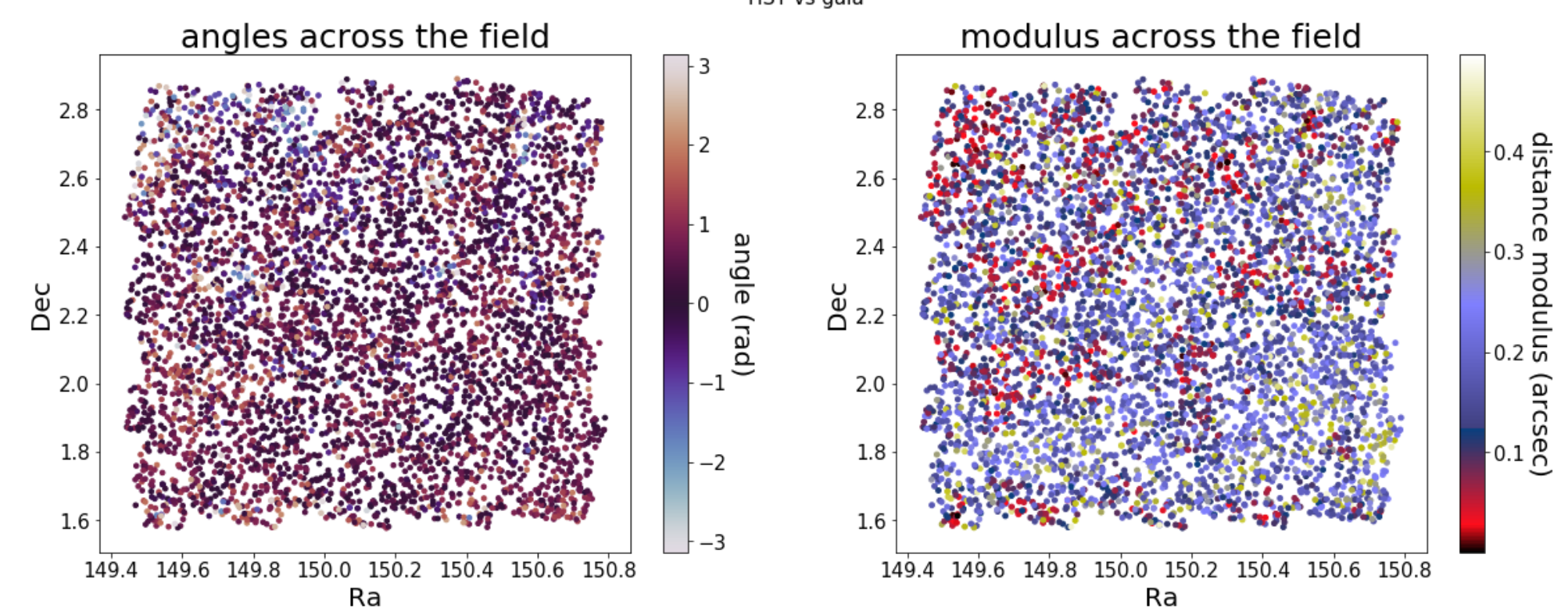
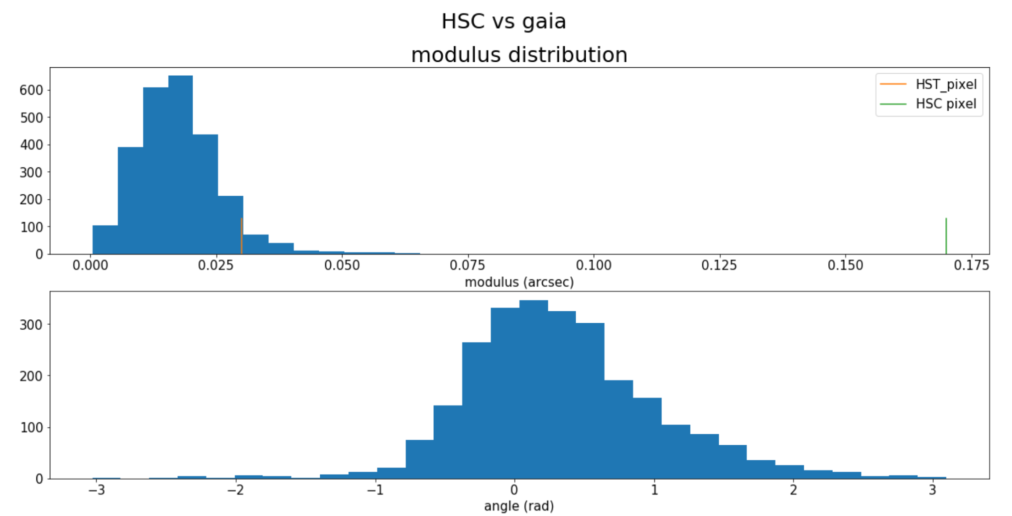
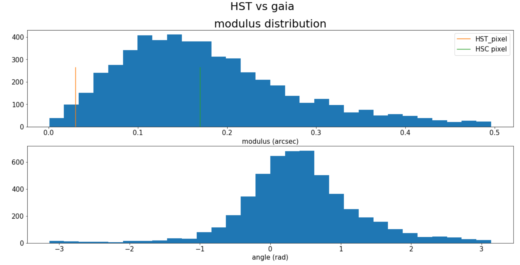
Astrometry
HSC s18 dud catalog
Gaia dr2
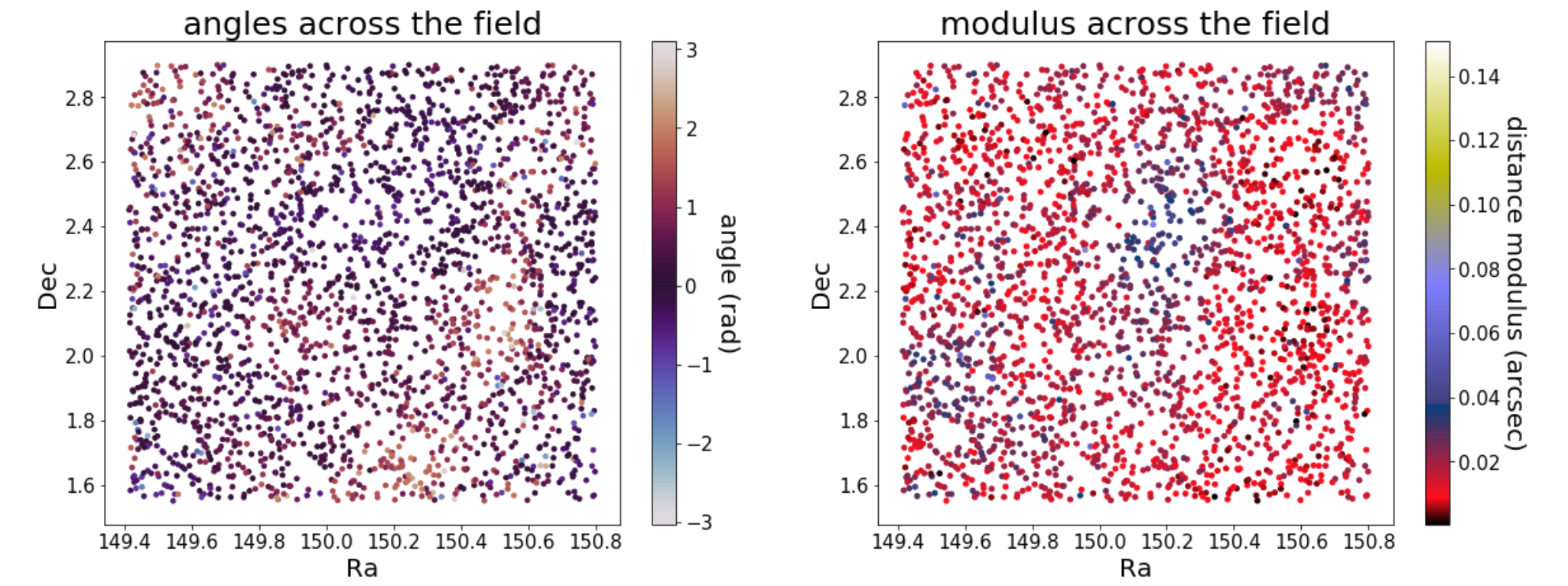
HSC - Gaia
HST - Gaia
HST cosmos, F814w
HSC DR2, grizy
Scarlet model
1
2
4
3
5
6
1
2
4
3
5
6
1
2
4
3
5
6
Multi-resolution in Scarlet
Takes advantage of both colour and resolution
To do:
- Improve simulations: realistic profiles, magnitudes
- Quantify the gain from multi-resolution detection
- Test multi-detection vs multi-resolution
- Quantify the allowed astrometric error
- Tests with BTK: New multi-resolution capabilities
- Allow PSFs to shift to alleviate astrometric errors
Interpolation kernel is actually a sinc
\(f_2(X) = (f_1*P)(X) = (\sum_{x_k} f_1(x_k)sinc(\frac{X-x_k}{h}))*(\sum_{x_p}P(x_p)sinc(\frac{X-x_p}{h}))\)
\(f_2(X) = (f_1*P)(X) = \sum_{x_k} f_1(x_k)\sum_{x_l}P(x_l)sinc(\frac{X-x_k - x_l}{h})\)
\(f_2(X) = (f_1*P)(X) = \sum_{x_k} f_1(x_k)\sum_{x_l}P(x_l- X)sinc(\frac{x_k + x_l}{h})\)
Making sure we get the pixel response right
\(I_2(x_{i2},y_{j2}).\) = \((rect_{h_1}*(f*p_1) *{F}^{-1}(\frac{\hat{rect_{h_2}}}{\hat{rect_{h_1}}}\frac{\hat{p_2}}{\hat{p_1}}))(x_{i2},y_{j2})\)
\(I_2(x_{i2},y_{j2}) = (rect_{h_2}*p_2*f)(x_{i2},y_{j2})\)
Multi-resolution Scarlet and LSBG deblending
By herjy


