NEURAL NETWORKS
and beyond....
Aadharsh Aadhithya A
Amrita Vishwa VIdhyapeetham
Center for Computational Engineering and Networking
NEURAL NETWORKS
and beyond....
- Introduction
- Perceptron
- Single-layered Neural Network
- Multi layered Neural Network
- Implicit Layers
- Implicit Function Theorem
- Opt Net
- Future Directions
Why NN???????
Why NN???????
What AI?
Why NN???????
What AI?
Goals Of AI??

Why NN???????
What AI?
Turings Test on Intellegence
What exactly is Intellegenceee??
Why NN???????
What AI?
Turings Test on Intellegence
Why NN are able to "Mimic Intelligence"
Why NN???????
What AI?
Turings Test on Intellegence
Are NN's Really Intellgent?

Why NN???????
What AI?
Are NN's Really Intellgent? No. Why Then?
Introduction
Introduction


Why Deep Learning?? (Applications)
What Are Neural Networks??

What Are Neural Networks??

Models, That mimic Human Intelligence?
How to mimic?
- Associations
- Connections

But, Where Are Associations Stored??
- By Mid 1800's, It was discovered that brain was made up of connected cells called "Neurons"
- Neurons Excite and Simulate each other.
- Neurons connect to other neurons. The processing/capacity of the brain is a function of these connections

MP Neuron


End to END Learning
End to END Learning
Learn mapping directly from input to output without the need for intermediate representations
Overcome cumbersome methods like feature extraction, multiple processing
steps.
End to END Learning

Perceptrons
Perceptrons
\Sigma
\int
\hat{y}
x_1
w_1
x_3
x_2
w_2
w_3
Perceptrons
\Sigma
\int
\hat{y}
x_1
w_1
x_3
x_2
w_2
w_3
\left ( \sum_{i = 1}^{m}x_i \cdot w_i \right )
Perceptrons
\Sigma
\int
\hat{y}
x_1
w_1
x_3
x_2
w_2
w_3
g \left ( \sum_{i = 1}^{m}x_i \cdot w_i \right )
Perceptrons
\Sigma
\int
\hat{y}
x_1
w_1
x_3
x_2
w_2
w_3
Perceptrons
\Sigma
\int
\hat{y}
x_1
w_1
x_3
x_2
w_2
w_3
Perceptrons
\Sigma
\int
\hat{y}
x_1
w_1
x_3
x_2
w_2
w_3
\hat{y} = g \left ( \sum_{i = 1}^{m}x_i \cdot w_i \right )
\text{Output}
\text{Aggregation}
\text{Non linear} \\ \text{Activation Function}
Single layer neural network
Single layer neural network
\Sigma
\int
\hat{y}
x_1
w_1
x_3
x_2
w_2
w_3
Single layer neural network
\Sigma
\int
\hat{y}
x_1
w_1
x_3
x_2
w_2
w_3
Single layer neural network
x_1
w_1
x_3
x_2
w_2
w_3
\hat{y}
g(z)
Single layer neural network
x_1
w_{11}
x_3
x_2
w_{12}
w_{13}
\hat{y}_1
g(z_{1})
\hat{y}_2
g(z_{2})
w_{21}
w_{22}
w_{23}
Single layer neural network
x_1
w_1
x_3
x_2
w_2
w_3
\hat{y}
g(z)
Single layer neural network
1
0.5
3
2
0.2
0.4
\hat{y}
g(z)
x = \begin{bmatrix} 1 \\ 2 \\ 3 \end{bmatrix} \\
y = 1 \\
\text{random weights , } \\
w = \begin{bmatrix} 0.5 \\ 0.2 \\ 0.4 \end{bmatrix} \\
Single layer neural network
1
0.5
3
2
0.2
0.4
\hat{y}
g(z)
x = \begin{bmatrix} 1 \\ 2 \\ 3 \end{bmatrix} \\
y = 1 \\
\text{random weights , } \\
w = \begin{bmatrix} 0.5 \\ 0.2 \\ 0.4 \end{bmatrix} \\
z = w^T \cdot x
[1 \cdot 0.5 + 2 \cdot 0.2 + 3 \cdot 0.4]
\text{z = 2.1}
Single layer neural network
\text{Activation Function}
Sigmoid Function

g(z) = \frac{1}{1 + e^{-z} }
g'(z) = g(z) \cdot (1 - g(z) )
Single layer neural network
g(z) = \frac{1}{1 + e^{-z} }
1
0.5
3
2
0.2
0.4
\hat{y}
g(z)
\text{z = 2.1}
\hat{y} = 0.8909
Single layer neural network
g(z) = \frac{1}{1 + e^{-z} }
1
0.5
3
2
0.2
0.4
\hat{y}
g(z)
\text{z = 2.1}
\hat{y} = 0.8909
OOPs! 🤥
Wasn't the true output 1?
Single layer neural network
g(z) = \frac{1}{1 + e^{-z} }
1
0.5
3
2
0.2
0.4
\hat{y}
g(z)
\text{z = 2.1}
\hat{y} = 0.8909
OOPs! 🤥
Wasn't the true output 1?
We Should Punish the Network , so
It Behaves Properly
Single layer neural network
g(z) = \frac{1}{1 + e^{-z} }
1
0.5
3
2
0.2
0.4
\hat{y}
g(z)
\text{z = 2.1}
\hat{y} = 0.8909
OOPs! 🤥
Wasn't the true output 1?
We Should Punish the Network , so
It Behaves Properly
LOSS FUNCTIONS
Answer:
Single layer neural network
LOSS FUNCTIONS
Binary Cross Entropy Loss
L(y , \hat{y}) = - y \cdot log(\hat{y} ) - (1-y) \cdot log(1 - \hat{y})
L(y , \hat{y} ) = \begin{cases}
- log(\hat{y}) && y == 1 \\
- log(1 - \hat{y}) && y == 0
\end{cases}
Judge?? Nah!, Classify 😎


y = 1 \\
L(y , \hat{y} ) = - log(\hat{y})
y = 0 \\
L(y, \hat{y}) = -log(1-\hat{y})
The Gradient of the Loss Function dictates whether to increase or decrease the wights and bias of a neural network
The Gradient of the Loss Function dictates whether to increase or decrease the wights and bias of a neural network
"Gradient" points up the curve in the increasing direction , so we need to move int the opposite direction
w = w + (-1) \cdot \alpha (\frac{\partial L(y,\hat{y} )}{\partial w})
\alpha \rightarrow scalar \rightarrow Learning \, Rate


Single layer neural network
1
0.5
3
2
0.2
0.4
g(z)
\text{z = 2.1}
\hat{y} = 0.8909
L(y , \hat{y})
L(y , \hat{y}) = - y \cdot log(\hat{y} ) - (1-y) \cdot log(1 - \hat{y})
Single layer neural network
1
0.5
3
2
0.2
0.4
g(z)
\text{z = 2.1}
\hat{y} = 0.8909
L(y , \hat{y}) = - y \cdot log(\hat{y} ) - (1-y) \cdot log(1 - \hat{y})
L(1 , 0.8009) = - 1 \cdot log(0.8909) - (1-1) \cdot log(1 - 0.8909)
Single layer neural network
1
0.5
3
2
0.2
0.4
g(z)
\text{z = 2.1}
\hat{y} = 0.8909
L(1 , 0.8009) = 0.1155
Single layer neural network
1
0.5
3
2
0.2
0.4
\text{z = 2.1}
\hat{y} = 0.8909
L(1 , 0.8009) = 0.1155
\frac{\partial L}{\partial \hat{y} }
\frac{\partial L}{\partial \hat{y}} = \frac{-y}{\hat{y}} + \frac{1 - y}{1 - \hat{y}}
\frac{ \partial L(1 , 0.8909) }{ \partial \hat{y}}= - \frac{1}{0.89} = -1.123
z
g(z)
Single layer neural network
1
0.5
3
2
0.2
0.4
\text{z = 2.1}
\hat{y} = 0.8909
L(1 , 0.8009) = 0.1155
\frac{\partial L}{\partial \hat{y} }=-1.123
z
g(z)
\frac{\partial L}{\partial z }
\frac{ \partial L} {\partial z} = \frac{\partial L}{\partial \hat{y}} \cdot \frac{\partial \hat{y}}{\partial z}
\left( -\frac{1} {\hat{y}} \right) \cdot \left( \hat{y} (1 - \hat{y}) \right)
-1.123 \cdot (0.8909(1-0.8909)) \\
= -0.1092
Single layer neural network
1
3
2
\text{z = 2.1}
\hat{y} = 0.8909
L(1 , 0.8009) = 0.1155
\frac{\partial L}{\partial \hat{y} }=-1.123
z
g(z)
\frac{\partial L}{\partial z } = -0.1092
\frac{\partial L}{\partial w_i} = \frac{\partial L}{\partial z} \cdot \frac{\partial z}{\partial w_i}
\frac{\partial z}{\partial w_i} =\frac{\partial \sum w_i x_i}{\partial w_i} = x_i
\frac{\partial L}{\partial w_1} = -0.1092*1 \\
\frac{\partial L}{\partial w_2} = -0.1092*2 \\
\frac{\partial L}{\partial w_3} = -0.1092*3 \\
\frac{\partial L}{\partial w_1}
\frac{\partial L}{\partial w_3}
\frac{\partial L}{\partial w_2}
Single layer neural network
\text{z = 2.1}
\hat{y} = 0.8909
L(1 , 0.8009) = 0.1155
\frac{\partial L}{\partial \hat{y} }=-1.123
\frac{\partial L}{\partial z } = -0.1092
\frac{\partial L}{\partial w_1} = -0.1092 \\
\frac{\partial L}{\partial w_2} = -0.2184 \\
\frac{\partial L}{\partial w_3} = -0.3276 \\
w_1 = w_1 - \alpha \cdot \frac{\partial L}{\partial w_1}
w_2 = w_2 - \alpha \cdot \frac{\partial L}{\partial w_2}
w_3 = w_3 - \alpha \cdot \frac{\partial L}{\partial w_3}
\alpha \rightarrow Learning \ rate
Single layer neural network
\text{z = 2.1}
\hat{y} = 0.8909
L(1 , 0.8009) = 0.1155
\frac{\partial L}{\partial \hat{y} }=-1.123
\frac{\partial L}{\partial z } = -0.1092
\frac{\partial L}{\partial w_1} = -0.1092 \\
\frac{\partial L}{\partial w_2} = -0.2184 \\
\frac{\partial L}{\partial w_3} = -0.3276 \\
w_1 = 0.5 - 1 \cdot (-0.1092)
w_2 = 0.2- 1 \cdot (-0.2184)
w_3 = 0.4- 1 \cdot (-0.3276)
\alpha \rightarrow Learning \ rate = 1
w_1 = 0.6092 \\
w_2 = 0.4184 \\
w_3 = 0.7276
Single layer neural network
x = \begin{bmatrix} 1 \\ 2 \\ 3 \end{bmatrix} \\
y = 1 \\
\text{updated weights , } \\
w = \begin{bmatrix} 0.6092 \\ 0.4184 \\ 0.7276 \end{bmatrix} \\
1
0.6092
3
2
0.4184
0.7276
\hat{y}
g(z)
z = w^T \cdot x
[1 \cdot 0.6092 + 2 \cdot 0.4184 + 3 \cdot 0.7276] \\
= 3.6288
g(z) = g(3.6288) = 0.9739
L(1, 0.9739) = 0.02
Old \ loss = 0.1155
Multi Layer Network
Multi Layer Network
x_1
w_{11}^1
x_3
x_2
w_{12}^1
w_{13}^1
g(z_{1})^1
g(z_{2})^1
w_{21}^1
w_{22}^1
w_{23}^1
w_{11}^2
w_{12}^2
g(z_{1})^2
\hat{y}
W^i = \begin{bmatrix}
w^i_{11} & w^i_{12} & w^i_{13} & \cdots&w^i_{1n} \\
w^i_{21} & w^i_{22} & w^i_{23} & \cdots&w^i_{2n} \\
\vdots & \ddots& \ddots & \vdots \\
w^i_{m1} & w^i_{m2} & w^i_{m3} & \cdots&w^i_{mn} \\
\end{bmatrix}
m \rightarrow \text{no .of neurons in } i^{th} \text{ layer} \\
n \rightarrow \text{no .of neurons in } (i-1)^{th} \text{ layer}
X^i = \begin{bmatrix}
x_1 \\
x_2\\
\vdots \\
x_n
\end{bmatrix}
X^i \rightarrow \text{Output of } (i-1)^{th} \text{ layer} \\
n \rightarrow \text{no .of neurons in } (i-1)^{th} \text{ layer}
b^i = \begin{bmatrix} b_1^i \\ b_2^i \\ \vdots \\ b_m^i \end{bmatrix}
Multi Layer Network
x_1
w_{11}^1
x_3
x_2
w_{12}^1
w_{13}^1
w_{21}^1
w_{22}^1
w_{23}^1
w_{11}^2
w_{12}^2
g(z_{1})^2
\hat{y}
\Sigma
\int
\Sigma\\
z_1
\Sigma \\ z_2
g(z_2)
g(z_`)
L(y,\hat{y})
Multi Layer Network
x_1
w_{11}^1
x_3
x_2
w_{12}^1
w_{13}^1
w_{21}^1
w_{22}^1
w_{23}^1
w_{11}^2
w_{12}^2
g(z_{1})^2
\hat{y}
\Sigma
\int
\Sigma\\
z_1
\Sigma \\ z_2
g(z_2)
g(z_`)
L(y,\hat{y})
Forward Pass
z^i = W^i \cdot x^i + b^i \\
y^i = g(z^i)
Multi Layer Network
x_1
w_{11}^1
x_3
x_2
w_{12}^1
w_{13}^1
w_{21}^1
w_{22}^1
w_{23}^1
w_{11}^2
w_{12}^2
g(z_{1})^2
\hat{y}
\Sigma
\int
\Sigma\\
z_1
\Sigma \\ z_2
g(z_2)
g(z_`)
L(y,\hat{y})
Forward Pass
z^1 = W^1 \cdot x^1 + b^1 \\
Multi Layer Network
x_1
w_{11}^1
x_3
x_2
w_{12}^1
w_{13}^1
w_{21}^1
w_{22}^1
w_{23}^1
w_{11}^2
w_{12}^2
g(z_{1})^2
\hat{y}
\Sigma
\int
\Sigma\\
z_1
\Sigma \\ z_2
g(z_2)
g(z_`)
L(y,\hat{y})
Forward Pass
y^1 = g(z^1)
Multi Layer Network
x_1
w_{11}^1
x_3
x_2
w_{12}^1
w_{13}^1
w_{21}^1
w_{22}^1
w_{23}^1
w_{11}^2
w_{12}^2
\hat{y}
L(y,\hat{y})
Forward Pass
\cdots \\
y^i = g(z^i)
g(z_{1})^1
g(z_{2})^1
\Sigma
\int
\Sigma\\
(z_1)^2
(g(z_1))^2
Multi Layer Network
x_1
w_{11}^1
x_3
x_2
w_{12}^1
w_{13}^1
w_{21}^1
w_{22}^1
w_{23}^1
w_{11}^2
w_{12}^2
\hat{y}
L(y,\hat{y})
Forward Pass
\cdots \\
y^i = g(z^i)
g(z_{1})^1
g(z_{2})^1
\Sigma
\int
\Sigma\\
(z_1)^2
(g(z_1))^2
Multi Layer Network
x_1
w_{11}^1
x_3
x_2
w_{12}^1
w_{13}^1
w_{21}^1
w_{22}^1
w_{23}^1
w_{11}^2
w_{12}^2
\hat{y}
L(y,\hat{y})
BackPropagation
\cdots \\
y^i = g(z^i)
g(z_{1})^1
g(z_{2})^1
\Sigma
\int
\Sigma\\
(z_1)^2
(g(z_1))^2
Multi Layer Network
x_1
x_3
x_2
w_{j k}^i
w_{11}^2
w_{12}^2
\hat{y}
L(y,\hat{y})
BackPropagation
\Sigma
\int
\Sigma\\
(z_1)^2
(g(z_1))^2
\Sigma
\int
\Sigma\\
z_1
\Sigma \\ z_2
g(z_2)
g(z_`)
w_{11}^1
w_{12}^1
w_{22}^1
w_{23}^1
\cdots
w_{j k}^i \rightarrow i^{th} \text{layer ,} j^{th} \text{neuron , mapping to } k^{th} \text{ input}
Multi Layer Network
x_1
x_3
x_2
w_{j k}^i
w_{11}^2
w_{12}^2
\hat{y}
L(y,\hat{y})
BackPropagation
\Sigma
\int
\Sigma\\
(z_1)^2
(g(z_1))^2
\Sigma
\int
\Sigma\\
z_1
\Sigma \\ z_2
g(z_2)
g(z_`)
w_{11}^1
w_{12}^1
w_{22}^1
w_{23}^1
\cdots
\frac{\partial L(y , \hat{y} )}{\partial w^i_{jk}}
Multi Layer Network
x_1
x_3
x_2
w_{j k}^i
w_{11}^2
w_{12}^2
\hat{y}
L(y,\hat{y})
BackPropagation
\Sigma
\int
\Sigma\\
(z_1)^2
(g(z_1))^2
\Sigma
\int
\Sigma\\
z_1
\Sigma \\ z_2
g(z_2)
g(z_`)
w_{11}^1
w_{12}^1
w_{22}^1
w_{23}^1
\cdots
\frac{\partial L(y , \hat{y} )}{\partial w^i_{jk}}
\text{changing } \hat{y} \text{ changes } L(y,\hat{y})
\frac{\partial L(y , \hat{y} )}{\partial \hat{y} } \frac{\partial \hat{y} }{\partial w^i_{jk}}
We can derive
To Be Computed
Here , We Can Resort To Using The Chain Rule .
How G changes with x?
Changing x changes h(x)
\frac{d h(x)}{dx}
Changing h changes g
\frac{d g}{dh}
\frac{dg} {dx} = \frac{d h(x)}{dx} \cdot \frac{d g}{dh}
Multi Layer Network
x_1
x_3
x_2
w_{j k}^i
w_{11}^2
w_{12}^2
\hat{y}
L(y,\hat{y})
BackPropagation
\Sigma
\int
\Sigma\\
(z_1)^2
(g(z_1))^2
\Sigma
\int
\Sigma\\
z_1
\Sigma \\ z_2
g(z_2)
g(z_`)
w_{11}^1
w_{12}^1
w_{22}^1
w_{23}^1
\cdots
\frac{\partial L(y , \hat{y} )}{\partial w^i_{jk}}
\text{How do we reach } w^i_{jk} \text{ From} L(y,\hat{y})
Multi Layer Network
x_1
x_3
x_2
w_{j k}^i
\hat{y}
L(y,\hat{y})
BackPropagation
\Sigma
\int
\Sigma\\
(z_1)^2
(g(z_1))^2
\Sigma
\int
\Sigma\\
z_1
\Sigma \\ z_2
g(z_2)
g(z_`)
w_{11}^1
w_{12}^1
w_{22}^1
w_{23}^1
\cdots
\frac{\partial L(y , \hat{y} )}{\partial w^i_{jk}}
\text{How do we reach } w^i_{jk} \text{ From } L(y,\hat{y}) ??
Follow The RED Path !
Multi Layer Network
x_1
x_3
x_2
w_{j k}^i
\hat{y}
L(y,\hat{y})
BackPropagation
\Sigma
\int
\Sigma\\
(z_1)^2
(g(z_1))^2
\Sigma
\int
\Sigma\\
z_1
\Sigma \\ z_2
g(z_2)
g(z_`)
w_{11}^1
w_{12}^1
w_{22}^1
w_{23}^1
\cdots
\frac{\partial L(y , \hat{y} )}{\partial w^i_{jk}}
\frac{\partial L(y,\hat{y})}{\partial \hat{y}}
\text{How } L(y , \hat{y} ) \text{ changes with } \hat{y}
Multi Layer Network
x_1
x_3
x_2
w_{j k}^i
\hat{y}
L(y,\hat{y})
BackPropagation
\Sigma
\int
\Sigma\\
(z_1)^2
(g(z_1))^2
\Sigma
\int
\Sigma\\
z_1
\Sigma \\ z_2
g(z_2)
g(z_`)
w_{11}^1
w_{12}^1
w_{22}^1
w_{23}^1
\cdots
\frac{\partial L(y , \hat{y} )}{\partial w^i_{jk}}
\frac{\partial L(y,\hat{y})}{\partial \hat{y}}
\text{How } \hat{y} \text{ changes with } (z_1)^{i+1}
\frac{\partial \hat{y}}{\partial (z_1)^{i+1}}
Multi Layer Network
x_1
x_3
x_2
w_{j k}^i
\hat{y}
L(y,\hat{y})
BackPropagation
\Sigma
\int
\Sigma\\
(z_1)^{i+1}
(g(z_1))^2
\Sigma
\int
\Sigma\\
z_1^i
\Sigma \\ z_2^i
g(z_2)^i
g(z_1)^i
w_{11}^1
w_{12}^1
w_{22}^1
w_{23}^1
\cdots
\frac{\partial L(y , \hat{y} )}{\partial w^i_{jk}}
\frac{\partial L(y,\hat{y})}{\partial \hat{y}}
\text{How } z_1^{i+1} \text{ changes with } g(z_i^i)
\frac{\partial \hat{y}}{\partial (z_1)^{i+1}}
\frac{\partial z_1^{i+1} }{\partial g(z_i^i)}
Multi Layer Network
x_1
x_3
x_2
w_{j k}^i
\hat{y}
L(y,\hat{y})
BackPropagation
\Sigma
\int
\Sigma\\
(z_1)^{i+1}
(g(z_1))^2
\Sigma
\int
\Sigma\\
z_1^i
\Sigma \\ z_2^i
g(z_2)^i
g(z_1)^i
w_{11}^1
w_{12}^1
w_{22}^1
w_{23}^1
\cdots
\frac{\partial L(y , \hat{y} )}{\partial w^i_{jk}}
\frac{\partial L(y,\hat{y})}{\partial \hat{y}}
\text{How } g(z_1)^i \text{ changes with } z_1^i
\frac{\partial \hat{y}}{\partial (z_1)^{i+1}}
\frac{\partial z_1^{i+1} }{\partial g(z_i^i)}
\frac{\partial g(z_1)^i }{\partial z_1^i}
Multi Layer Network
x_1
x_3
x_2
w_{j k}^i
\hat{y}
L(y,\hat{y})
BackPropagation
\Sigma
\int
\Sigma\\
(z_1)^{i+1}
(g(z_1))^2
\Sigma
\int
\Sigma\\
z_1^i
\Sigma \\ z_2^i
g(z_2)^i
g(z_1)^i
w_{11}^1
w_{12}^1
w_{22}^1
w_{23}^1
\cdots
\frac{\partial L(y , \hat{y} )}{\partial w^i_{jk}}
\frac{\partial L(y,\hat{y})}{\partial \hat{y}}
\text{How } z_1^i \text{ changes with } w^i_{jk}
\frac{\partial \hat{y}}{\partial (z_1)^{i+1}}
\frac{\partial z_1^{i+1} }{\partial g(z_i^i)}
\frac{\partial g(z_1)^i }{\partial z_1^i}
\frac{\partial z_1^i}{\partial w^i_{jk}}
Multi Layer Network
x_1
x_3
x_2
w_{j k}^i
\hat{y}
L(y,\hat{y})
BackPropagation
\Sigma
\int
\Sigma\\
(z_1)^{i+1}
(g(z_1))^2
\Sigma
\int
\Sigma\\
z_1^i
\Sigma \\ z_2^i
g(z_2)^i
g(z_1)^i
w_{11}^1
w_{12}^1
w_{22}^1
w_{23}^1
\cdots
\frac{\partial L(y , \hat{y} )}{\partial w^i_{jk}} =
\frac{\partial L(y,\hat{y})}{\partial \hat{y}}
\text{How } L(y,\hat{y} ) \text{ changes with } w^i_{jk}
\frac{\partial \hat{y}}{\partial (z_1)^{i+1}}
\frac{\partial z_1^{i+1} }{\partial g(z_i^i)}
\frac{\partial g(z_1)^i }{\partial z_1^i}
\frac{\partial z_1^i}{\partial w^i_{jk}}
\frac{\partial z_1^i}{\partial w^i_{jk}}
\frac{\partial g(z_1)^i }{\partial z_1^i}
\frac{\partial z_1^{i+1} }{\partial g(z_i^i)}
\frac{\partial \hat{y}}{\partial (z_1)^{i+1}}
\frac{\partial L(y,\hat{y})}{\partial \hat{y}}
Multi Layer Network
BackPropagation
\frac{\partial L(y , \hat{y} )}{\partial w^i_{jk}} =
\frac{\partial z_1^i}{\partial w^i_{jk}}
\frac{\partial g(z_1)^i }{\partial z_1^i}
\frac{\partial z_1^{i+1} }{\partial g(z_i^i)}
\frac{\partial \hat{y}}{\partial (z_1)^{i+1}}
\frac{\partial L(y,\hat{y})}{\partial \hat{y}}
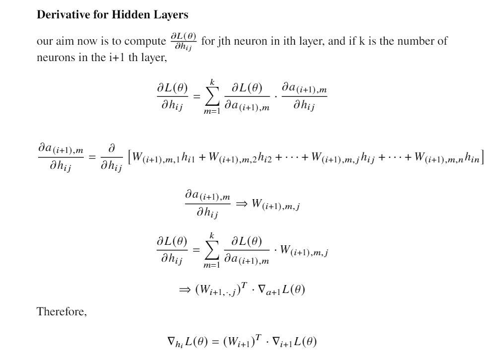
\text{ This is for one weights } w_{jk}^i \\ \text{for the matrix } W^i \text{ We Have a Detailed Derivation in the accompanying material}
(Project report)
For Softmax output layer and Sigmoid Activation function
Multi Layer Network
BackPropagation
Source : Project Report , Group01.pdf
Multi Layer Network
BackPropagation

Source : Project Report , Group01.pdf
Multi Layer Network
BackPropagation

Source : Project Report , Group01.pdf
Multi Layer Network
BackPropagation
So , now , we have all the vectorized components to build our chain

Source : Project Report , Group01.pdf
Multi Layer Network
Full Story

Source : Project Report , Group01.pdf
Multi Layer Network
import numpy as np  # import numpy library
from util.paramInitializer import initialize_parameters  # import function to initialize weights and biases


class LinearLayer:
    """
        This Class implements all functions to be executed by a linear layer
        in a computational graph

        Args:
            input_shape: input shape of Data/Activations
            n_out: number of neurons in layer
            ini_type: initialization type for weight parameters, default is "plain"
                      Opitons are: plain, xavier and he

        Methods:
            forward(A_prev)
            backward(upstream_grad)
            update_params(learning_rate)

    """

    def __init__(self, input_shape, n_out, ini_type="plain"):
        """
        The constructor of the LinearLayer takes the following parameters

        Args:
            input_shape: input shape of Data/Activations
            n_out: number of neurons in layer
            ini_type: initialization type for weight parameters, default is "plain"
        """

        self.m = input_shape[1]  # number of examples in training data
        # `params` store weights and bias in a python dictionary
        self.params = initialize_parameters(input_shape[0], n_out, ini_type)  # initialize weights and bias
        self.Z = np.zeros((self.params['W'].shape[0], input_shape[1]))  # create space for resultant Z output

    def forward(self, A_prev):
        """
        This function performs the forwards propagation using activations from previous layer

        Args:
            A_prev:  Activations/Input Data coming into the layer from previous layer
        """

        self.A_prev = A_prev  # store the Activations/Training Data coming in
        self.Z = np.dot(self.params['W'], self.A_prev) + self.params['b']  # compute the linear function

    def backward(self, upstream_grad):
        """
        This function performs the back propagation using upstream gradients

        Args:
            upstream_grad: gradient coming in from the upper layer to couple with local gradient
        """

        # derivative of Cost w.r.t W
        self.dW = np.dot(upstream_grad, self.A_prev.T)

        # derivative of Cost w.r.t b, sum across rows
        self.db = np.sum(upstream_grad, axis=1, keepdims=True)

        # derivative of Cost w.r.t A_prev
        self.dA_prev = np.dot(self.params['W'].T, upstream_grad)

    def update_params(self, learning_rate=0.1):
        """
        This function performs the gradient descent update

        Args:
            learning_rate: learning rate hyper-param for gradient descent, default 0.1
        """
        self.params['W'] = self.params['W'] - learning_rate * self.dW  # update weights
        self.params['b'] = self.params['b'] - learning_rate * self.db  # update bias(es)
Multi Layer Network
import numpy as np  # import numpy library


class SigmoidLayer:
    """
    This file implements activation layers
    inline with a computational graph model

    Args:
        shape: shape of input to the layer

    Methods:
        forward(Z)
        backward(upstream_grad)

    """

    def __init__(self, shape):
        """
        The consturctor of the sigmoid/logistic activation layer takes in the following arguments

        Args:
            shape: shape of input to the layer
        """
        self.A = np.zeros(shape)  # create space for the resultant activations

    def forward(self, Z):
        """
        This function performs the forwards propagation step through the activation function

        Args:
            Z: input from previous (linear) layer
        """
        self.A = 1 / (1 + np.exp(-Z))  # compute activations

    def backward(self, upstream_grad):
        """
        This function performs the  back propagation step through the activation function
        Local gradient => derivative of sigmoid => A*(1-A)

        Args:
            upstream_grad: gradient coming into this layer from the layer above

        """
        # couple upstream gradient with local gradient, the result will be sent back to the Linear layer
        self.dZ = upstream_grad * self.A*(1-self.A)
Multi Layer Network
def compute_stable_bce_cost(Y, Z):
    """
    This function computes the "Stable" Binary Cross-Entropy(stable_bce) Cost and returns the Cost and its
    derivative w.r.t Z_last(the last linear node) .
    The Stable Binary Cross-Entropy Cost is defined as:
    => (1/m) * np.sum(max(Z,0) - ZY + log(1+exp(-|Z|)))
    Args:
        Y: labels of data
        Z: Values from the last linear node

    Returns:
        cost: The "Stable" Binary Cross-Entropy Cost result
        dZ_last: gradient of Cost w.r.t Z_last
    """
    m = Y.shape[1]

    cost = (1/m) * np.sum(np.maximum(Z, 0) - Z*Y + np.log(1+ np.exp(- np.abs(Z))))
    dZ_last = (1/m) * ((1/(1+np.exp(- Z))) - Y)  # from Z computes the Sigmoid so P_hat - Y, where P_hat = sigma(Z)

    return cost, dZ_last
Multi Layer Network
def data_set(n_points, n_classes):
  x = np.random.uniform(-1,1, size=(n_points, n_classes)) # Generate (x,y) points
  mask = np.logical_or ( np.logical_and(x[:,0] > 0.0, x[:,1] > 0.0),  np.logical_and(x[:,0] < 0.0, x[:,1] < 0.0)) # True for 1st & 3rd quadrants
  y = 1*mask
  return x,y


no_of_points = 10000
no_of_classes = 2
X_train, Y_train = data_set(no_of_points, no_of_classes)


for i in range(10):
    print(f'The point is {X_train[i,0]} , {X_train[i,1]} and the class is {Y_train[i]}')


Multi Layer Network
# define training constants
learning_rate = 0.6
number_of_epochs = 5000

np.random.seed(48) # set seed value so that the results are reproduceable
                  # (weights will now be initailzaed to the same pseudo-random numbers, each time)


# Our network architecture has the shape:
#                   (input)--> [Linear->Sigmoid] -> [Linear->Sigmoid] -->(output)

#------ LAYER-1 ----- define hidden layer that takes in training data
Z1 = LinearLayer(input_shape=X_train.shape, n_out=4, ini_type='xavier')
A1 = SigmoidLayer(Z1.Z.shape)

#------ LAYER-2 ----- define output layer that takes in values from hidden layer
Z2= LinearLayer(input_shape=A1.A.shape, n_out= 1, ini_type='xavier')
A2= SigmoidLayer(Z2.Z.shape)
Multi Layer Network
costs = [] # initially empty list, this will store all the costs after a certian number of epochs

# Start training
for epoch in range(number_of_epochs):

    # ------------------------- forward-prop -------------------------
    Z1.forward(X_train)
    A1.forward(Z1.Z)

    Z2.forward(A1.A)
    A2.forward(Z2.Z)

    # ---------------------- Compute Cost ----------------------------
    cost, dZ2 = compute_stable_bce_cost(Y_train, Z2.Z)

    # print and store Costs every 100 iterations and of the last iteration.
    if (epoch % 100) == 0:
        print("Cost at epoch#{}: {}".format(epoch, cost))
        costs.append(cost)

    # ------------------------- back-prop ----------------------------

    Z2.backward(dZ2)

    A1.backward(Z2.dA_prev)
    Z1.backward(A1.dZ)

    # ----------------------- Update weights and bias ----------------
    Z2.update_params(learning_rate=learning_rate)
    Z1.update_params(learning_rate=learning_rate)

#     if (epoch % 100) == 0:
#         plot_decision_boundary(lambda x: predict_dec(Zs=[Z1, Z2], As=[A1, A2], X=x.T, thresh=0.5),  X=X_train.T, Y=Y_train , save=True)
Multi Layer Network

Multi Layer Network
def predict_loc(X, Zs, As, thresh=0.5):
    """
    helper function to predict on data using a neural net model layers

    Args:
        X: Data in shape (features x num_of_examples)
        Y: labels in shape ( label x num_of_examples)
        Zs: All linear layers in form of a list e.g [Z1,Z2,...,Zn]
        As: All Activation layers in form of a list e.g [A1,A2,...,An]
        thresh: is the classification threshold. All values >= threshold belong to positive class(1)
                and the rest to the negative class(0).Default threshold value is 0.5
    Returns::
        p: predicted labels
        probas : raw probabilities
        accuracy: the number of correct predictions from total predictions
    """
    m = X.shape[1]
    n = len(Zs)  # number of layers in the neural network
    p = np.zeros((1, m))

    # Forward propagation
    Zs[0].forward(X)
    As[0].forward(Zs[0].Z)
    for i in range(1, n):
        Zs[i].forward(As[i-1].A)
        As[i].forward(Zs[i].Z)
    probas = As[n-1].A

    # convert probas to 0/1 predictions
    for i in range(0, probas.shape[1]):
        if probas[0, i] >= thresh:  # 0.5  the default threshold
            p[0, i] = 1
        else:
            p[0, i] = 0

    # print results
    print ("predictions: " + str(p))
Multi Layer Network

Implicit Layers
Implicit Layers
z_{i+1} = f(z_i)
f(z_i , z_{i+1}) = 0
Explicit Layers
Implicit Layers
Implicit Layers
But Why?? 😕
Implicit Layers
But Why?? 😕
"Instead of specifying how to compute the layer's output from the input , we specify the conditions that we want the layer's output to satisfy"
Implicit Layers
But Why?? 😕
Recent Years Have seen several Efficient ways to Differentiate through constructs like Argmin and Argmax
argmin \, \, f(z_i , z_{i+1})
then , Backpropagation Requires Gradients
\frac{\partial}{\partial z_{i}} \, \, f(z_i , z_{i+1})
1.
Gould, S. et al. On Differentiating Parameterized Argmin and Argmax Problems with Application to Bi-level Optimization. arXiv:1607.05447 [cs, math] (2016).
Implicit Layers
But How?? 😕
Differentiating Through Implicit Layers?? 🤔
Implicit Layers
But Why?? 😕
Differentiating Through Implicit Layers?? 🤔
The Implicit Function Theorem
Implicit Layers
The Implicit Function Theorem
f : \mathbb{R}^n \times \mathbb{R}^m \rightarrow \mathbb{R}^m
Implicit Layers
The Implicit Function Theorem
f : \mathbb{R}^n \times \mathbb{R}^m \rightarrow \mathbb{R}^m
\text{for some} , a_0 \epsilon \mathbb{R}^n \,\, z_0 \epsilon \mathbb{R}^m \\
f(a_0 , z_0) = 0 \\
\text{f is continuously differentiable with non singular jacobian} \frac{\partial f(a_0 , z_0)}{\partial a_0}
Then the Implicit function theorem tells ,
\text{There Exists a local function } z^* \text{ such that}
z_0 = z^*(a_0) \\
f(a,z^*(a)) = 0 \forall a \, in \, the \, neighbourhood \\
z^* \, is \, differentiable \, in \, the \, neighbourhood
Implicit Layers
The Implicit Function Theorem
f : \mathbb{R}^n \times \mathbb{R}^m \rightarrow \mathbb{R}^m
Now , we know that there exists a local function z*,
f(a , z^*(a)) = 0 \, \forall \, \epsilon S_{a_0} \\
\frac{\partial f(a , z^*(a)) }{\partial a} + \frac{\partial f(a , z^*(a)) }{\partial z^*(a)} \frac{\partial z^*(a)}{\partial a} = 0 \, \, \, \forall a \epsilon S_{a_0}
S_{a_0} \text{Is the set of a's in the neighbourhood of } a_0 \text{ such that}
f(a , z^*(a)) = 0 \, \forall a \epsilon S_{a_0}
\frac{\partial z^*(a_0)}{\partial a} = - \left [ \frac{\partial f(a_0 , z^*(a_0)) }{\partial z^*(a)} \right ]^{-1} \frac{\partial f(a_0 , z^*(a_0)) }{\partial a}
Implicit Layers
The Implicit Function Theorem
f : \mathbb{R}^n \times \mathbb{R}^m \rightarrow \mathbb{R}^m
\frac{\partial z^*(a_0)}{\partial a} = - \left [ \frac{\partial f(a_0 , z^*(a_0)) }{\partial z^*(a)} \right ]^{-1} \frac{\partial f(a_0 , z^*(a_0)) }{\partial a}
\text{For Fixed Point solution mappings } f(a , z^*(a) ) = z_0 , \text{ This can be extended as , }
\frac{\partial f(a , z^*(a)) }{\partial a} + \frac{\partial f(a , z^*(a)) }{\partial z^*(a)} \frac{\partial z^*(a)}{\partial a} = z_0 \, \, \, \forall a \epsilon S_{a_0}
\frac{\partial z^*(a_0)}{\partial a} = \left [ I - \frac{\partial f(a_0 , z^*(a_0)) }{\partial z^*(a)} \right ]^{-1} \frac{\partial f(a_0 , z^*(a_0)) }{\partial a}
Implicit Layers
The Implicit Function Theorem
\frac{\partial z^*(a_0)}{\partial a} = \left [ I - \frac{\partial f(a_0 , z^*(a_0)) }{\partial z^*(a)} \right ]^{-1} \frac{\partial f(a_0 , z^*(a_0)) }{\partial a}
Now this can be connected to standard auto diffs tools..
Implicit Layers
Implicit Layers , Bring In Structure to the layers.
Encode Domain knowledge
Differentiable Optimization
Implicit Layers
Implicit Layers , Bring In Structure to the layers.
Encode Domain knowledge
Differentiable Optimization
z^* = argmin f(z,x) \, \, z \epsilon \textit{Constraint \, Set}(x)
Implicit Layers
OPTNET
Amos, Brandon, and J. Zico Kolter. 2019. OptNet: Differentiable Optimization as a Layer inNeural Networks.arXiv:1703.00443 [cs, math, stat](14 October 2019). arXiv: 1703.00443
z^* = argmin \, \, \frac{1}{2} z^T Q(x) z + p(z)^Tz \\ subject \, \, to \, \, \, \, A(x) z = b(x) \\ G(x)z \leq h(x)
Implicit Layers
OPTNET
z^* = argmin \, \, \frac{1}{2} z^T Q(x) z + p(z)^Tz \\ subject \, \, to \, \, \, \, A(x) z = b(x) \\ G(x)z \leq h(x)
KKT Conditions
"Necessary and Sufficient
Conditions for optimality "
( z^* , \nu^* , \lambda^*)
Implicit Form
Implicit Function Theorem
Implicit Layers
Our Trails And Fails
Implicit Layers
Our Trails And Fails
Adrian-Vasile Duka,
Neural Network based Inverse Kinematics Solution for Trajectory Tracking of a Robotic Arm,
Procedia Technology,Volume 12, 2014, Pages 20-27, ISSN 2212-0173,
https://doi.org/10.1016/j.protcy.2013.12.451.
(https://www.sciencedirect.com/science/article/pii/S2212017313006361)
Abstract: Planar two and three-link manipulators are often used in Robotics as testbeds for various algorithms or theories. In this paper, the case of a three-link planar manipulator is considered. For this type of robot a solution to the inverse kinematics problem, needed for generating desired trajectories in the Cartesian space (2D) is found by using a feed-forward neural network.
Keywords: robotic arm; planar manipulator; inverse kinematics; trajectory; neural networks
Adrian-VasileDuka Showed Training Neural Networks , for inverse kinematics , for a planar 3 link manipulator based on input - end effector coordinates using 1 hidden layer and 100 neurons
Implicit Layers
Our Trails And Fails
We Tried to Simulate Obstacle , by removing a circular region from randomly generated data..
Then Tried Appending the previous architecture with an optnet layer.
Implicit Layers
Our Trails And Fails
We Tried to Simulate Obstacle , by removing a circular region from randomly generated data..
Then Tried Appending the previous architecture with an optnet layer.
But we hit a roadblock..
class Link3IK(nn.Module):

def __init__(self,n,m,p):
    super().__init__()
    torch.manual_seed(0)
    z = cp.Variable(n)
    self.P = cp.Parameter((n,n))
    self.q = cp.Parameter(n)
    self.G = cp.Parameter((m,n))
    self.h = cp.Parameter(m)
    self.A = cp.Parameter((p,n))
    self.b = cp.Parameter(p)
    self.nn_output = cp.Parameter(3)

    scale_factor = 1e-4
    self.Ptch = torch.nn.Parameter(scale_factor*torch.randn(n,n))
    self.qtch = torch.nn.Parameter(scale_factor*torch.randn(n))
    self.Gtch = torch.nn.Parameter(scale_factor*torch.randn(m,n))
    self.htch = torch.nn.Parameter(scale_factor*torch.randn(m))
    self.Atch = torch.nn.Parameter(scale_factor*torch.randn(p,n))
    self.btch = torch.nn.Parameter(scale_factor*torch.randn(p))

    self.objective = cp.Minimize(0.5*cp.sum_squares(self.P @ self.z) + self.q @ self.z )
    self.constraints = [self.G@self.z-self.h <= 0 , self.A@self.z == self.b]
    raise NotImplementedError # include nn_output in the cvxpy problem.
    self.problem = cp.Problem(self.objective, self.constraints)
    self.net = nn.Sequential(
        nn.Linear(2, 100),
        nn.Sigmoid(),
        nn.Linear(100, 3),
        nn.Softmax()
    )
    self.cvxpylayer = CvxpyLayer(self.problem, parameters=[self.P,self.q,self.G,self.h,self.A,self.b,self.nn_output], variables=[self.z])

def forward(self, X):
    nn_output = self.net(X)
    output = self.cvxpylayer(self.Ptch, self.qtch, self.Gtch, self.htch, self.Atch, self.btch, nn_output)[0]
    return output
In order to include nn_output , we needed knowledge about convex spaces.. 😔
Future Potential Prospects
1.
Maric, F., Giamou, M., Khoubyarian, S., Petrovic, I. & Kelly, J. Inverse Kinematics for Serial Kinematic Chains via Sum of Squares Optimization. 2020 IEEE International Conference on Robotics and Automation (ICRA) 7101–7107 (2020) doi:10.1109/ICRA40945.2020.9196704.
Maric et al ., Casted Inverse kinematics as a sum of squares QCQP problem and solved using a custom solver
We could use that formulation to solve these problems using CVXPYlayers
Based On our understanding....
Future Potential Prospects
1.
Maric, F., Giamou, M., Khoubyarian, S., Petrovic, I. & Kelly, J. Inverse Kinematics for Serial Kinematic Chains via Sum of Squares Optimization. 2020 IEEE International Conference on Robotics and Automation (ICRA) 7101–7107 (2020) doi:10.1109/ICRA40945.2020.9196704.
- Reinforcement Learning
Learning Constraints in the state space
- Control
Things like LQE for Starting
Based On our understanding....
Role of BIAS
Role of BIAS
- Introduce an additional degree of freedom
- Offset any systematic errors or inconsistencies in the data
- Shift the decision boundary and better fit the training data
- In case of class imbalance shift decision boundary towards the minority class
Bias Variance Tradeoff
Bias Variance Tradeoff
Minimize both bias and
variance to achieve optimal predictive performance
High Bias
- Underfits the data
- Cannot capture complexity
- Poor predictive performance
High Variance
- Sensitive to data fluctuations
- Fits noise and underlying patterns
- Poor performance on unseen data
Bias Variance Tradeoff
Right balance for optimal performance
Regularization,
cross-validation, and Ensembling
Vanishing Gradient Problem
Vanishing Gradient Problem
Gradient of loss function w.r.t weights become very small
Prevalent in deeper networks as gradient is propagated through multiple layers making it smaller
Weights in earlier layers do not receive sufficient updates
Vanishing Gradient Problem
Activation functions like sigmoid have limited range causing derivatives to be mall for large inputs
Initialising small weights can make the gradients smaller
Vanishing Gradient Problem
Solution
ReLU, weight initialisation methods
(Xavier Initialisation)
Skip connections,
which allow the gradient to bypass some of the layers and propagate more directly to the earlier layers.
Advantages of Deeper Networks
Advantages of Deeper Networks
- Increased Representational Power
Learn Complex features
- Improved Feature Extraction
Lower layers can learn basic features while higher layers learn abstract features
More discrimination of features
- Better Generalization
Can filter noise and focus on genaralising patterns
Thank You!
DeepLearnong
By Incredeble us


