


He Wang PRO
Knowledge increases by sharing but not by saving.
He Wang (王赫)
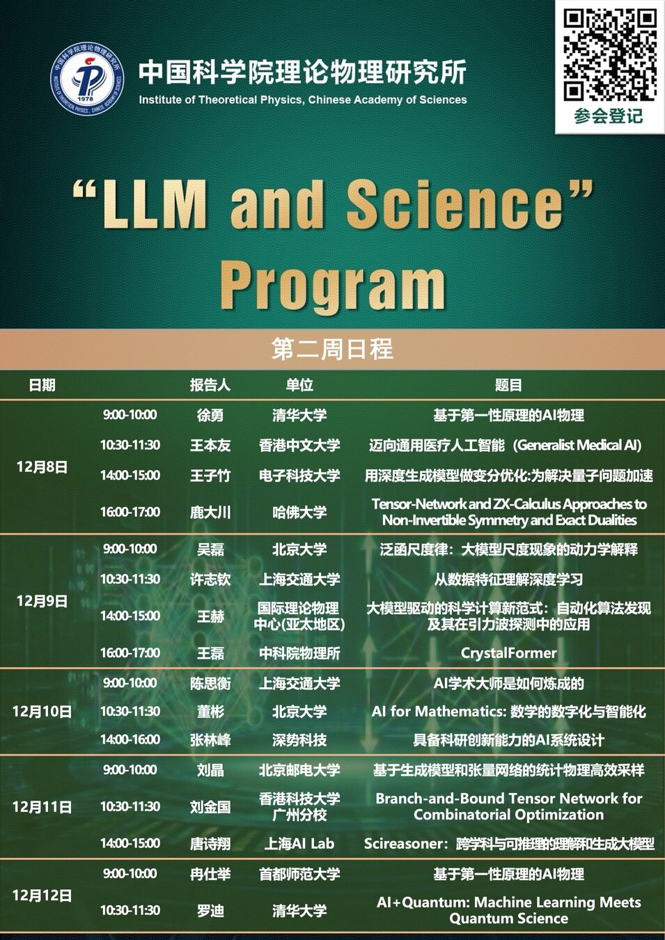
9th Dec 2025, 14:00-15:00. "LLM and Science" Program @ITP-CAS
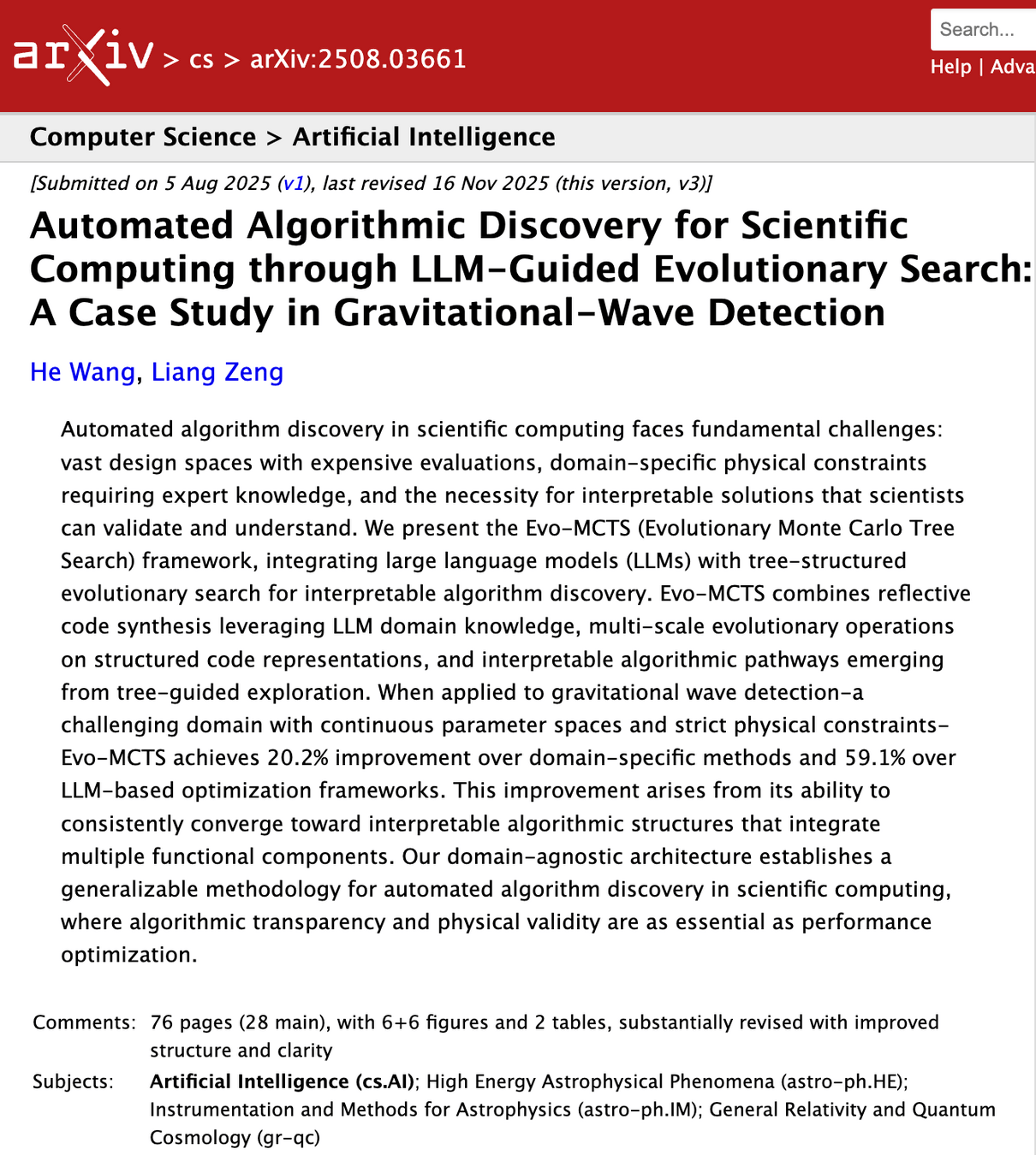
Based on arXiv:2508.03661, etc.
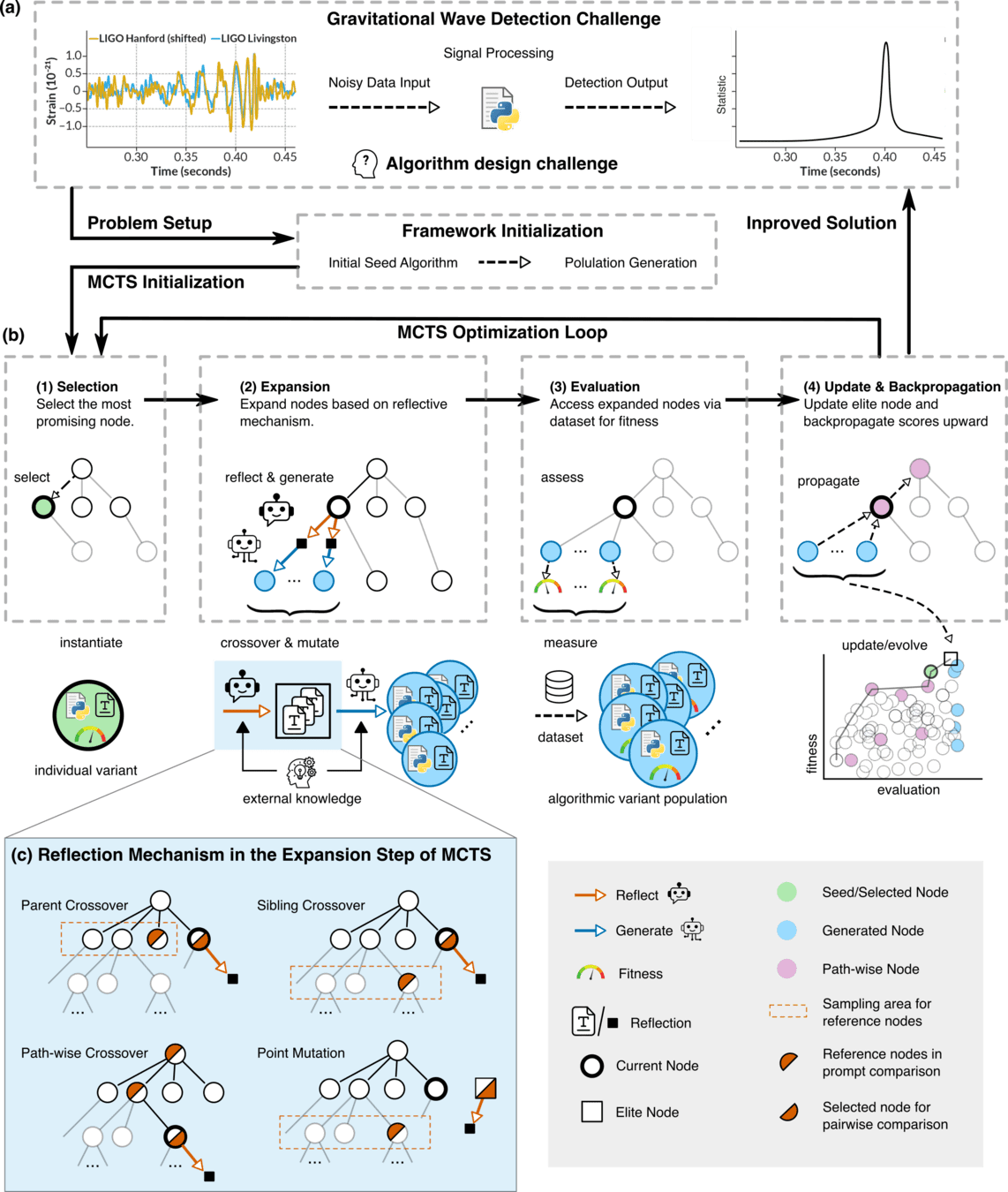
Interpretable Gravitational Wave Data Analysis with Reinforcement Learning and Large Language Models
hewang@ucas.ac.cn
International Centre for Theoretical Physics Asia-Pacific (ICTP-AP), UCAS
Taiji Laboratory for Gravitational Wave Universe (Beijing/Hangzhou), UCAS
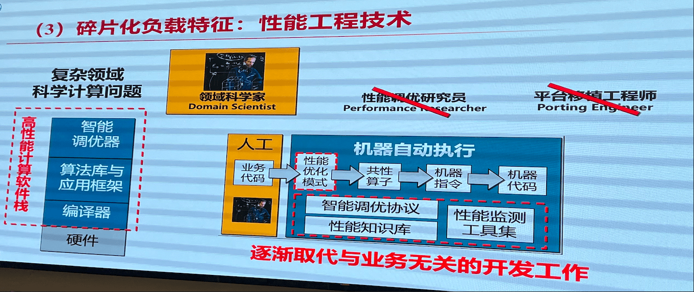
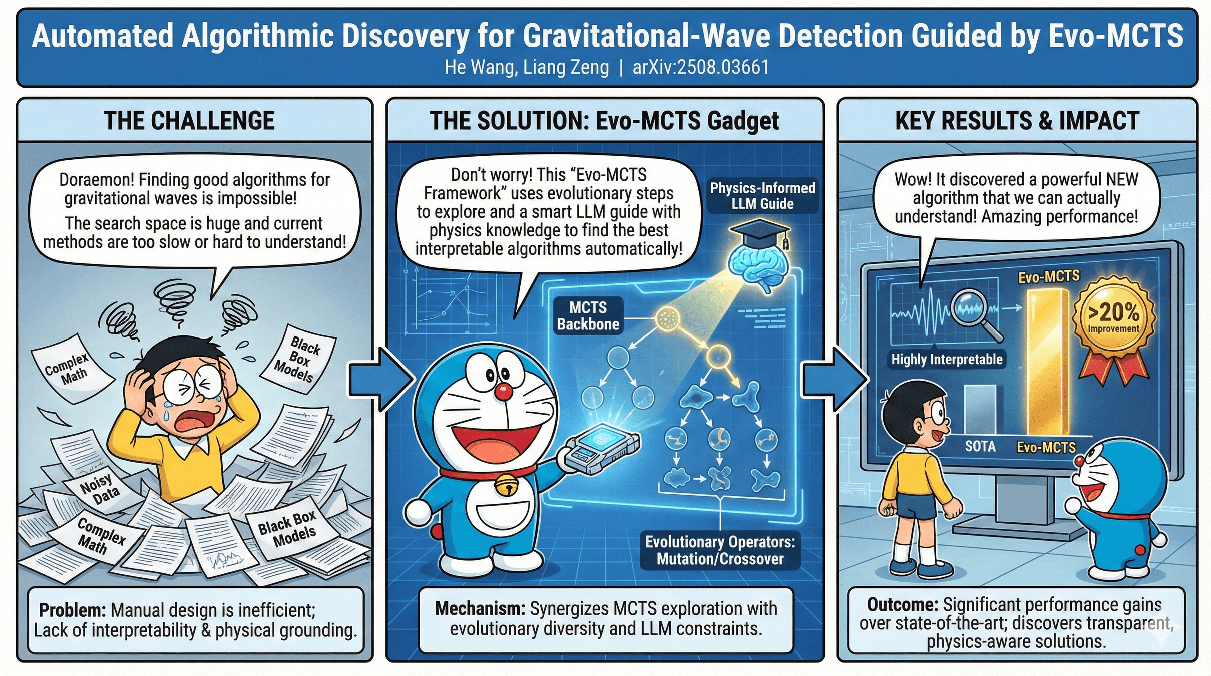
大语言模型(LLM)正为科学计算方法的设计与创新开辟新的路径。本报告介绍 Evo-MCTS 框架,其结合LLM的反思式代码生成与基于 MCTS 的结构化演化搜索,实现科学计算中的自动化算法发现。以引力波探测为测试场景,Evo-MCTS 在无需强人工先验的条件下生成可解释且物理一致的算法结构,并在基准任务上较领域特定方法提升 20.2%,较现有 LLM 优化框架提升 59.1%,同时能够稳定收敛到融合多种功能组件的高性能且可解释的算法结构。该研究展示了 LLM 主导的算法创新在科学计算中的潜力,并指向科研范式向自动化与模型共创方向的转变。
Uncovering the "black box" to reveal how AI actually works
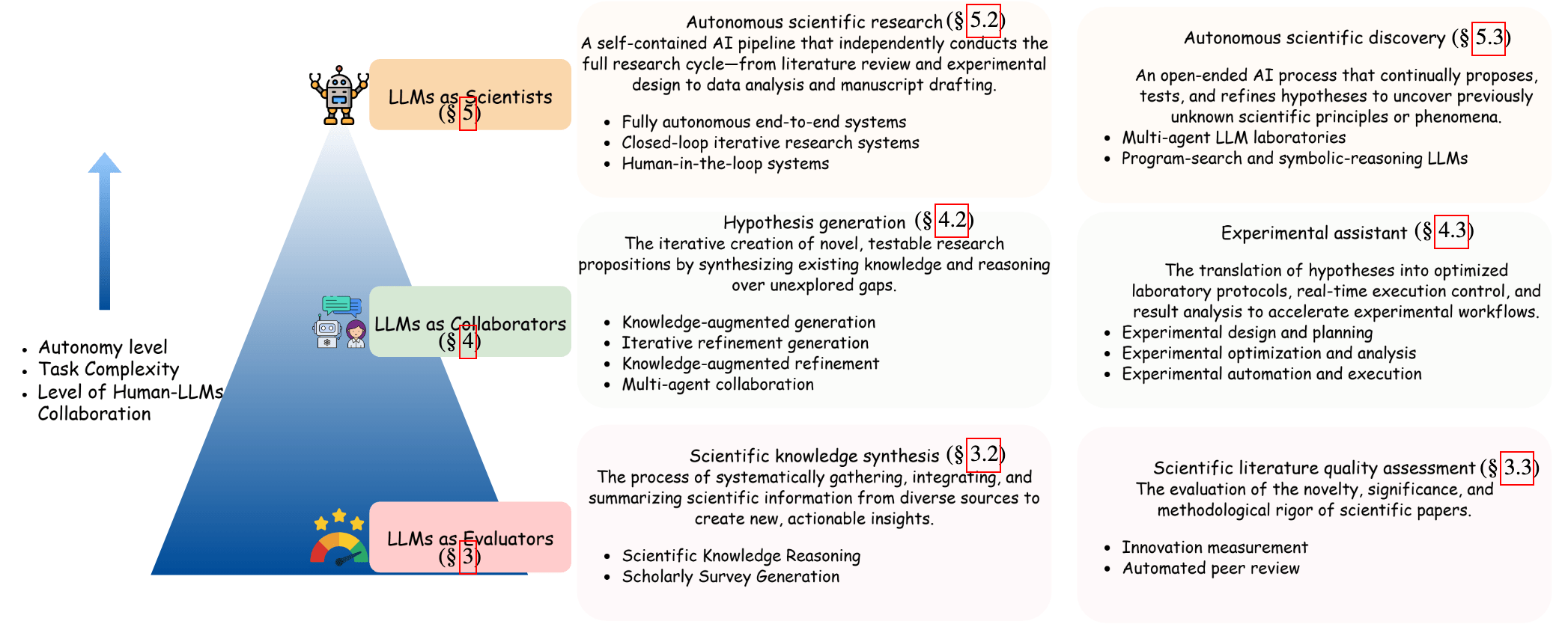
arXiv:2507.11810 [cs.DL]
"科学家"
"合作者"
"评估者"
Let's be honest about our motivations... 😉
npj Artif. Intell. 1, 14 (2025).
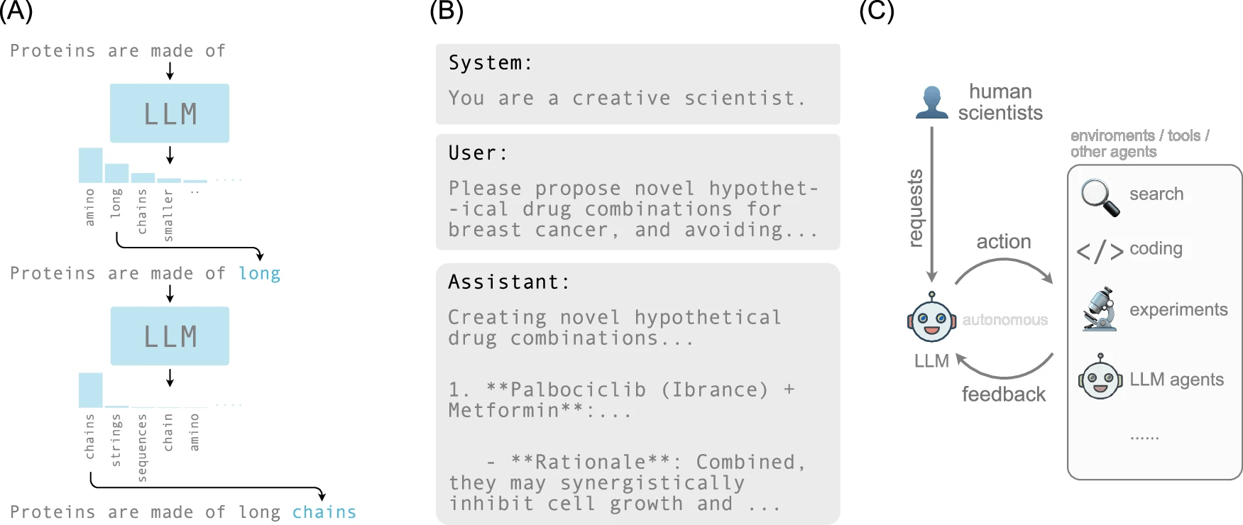
"序列生成"
"序列输入"
"Direct fails. Refine and recover."
直接不行?那就包装回炉再来一遍。
Let's be honest about our motivations... 😉
Let's be honest about our motivations... 😉
Generative agents rely on predefined rules. 🤫
arXiv:2304.03442 [cs.HC]
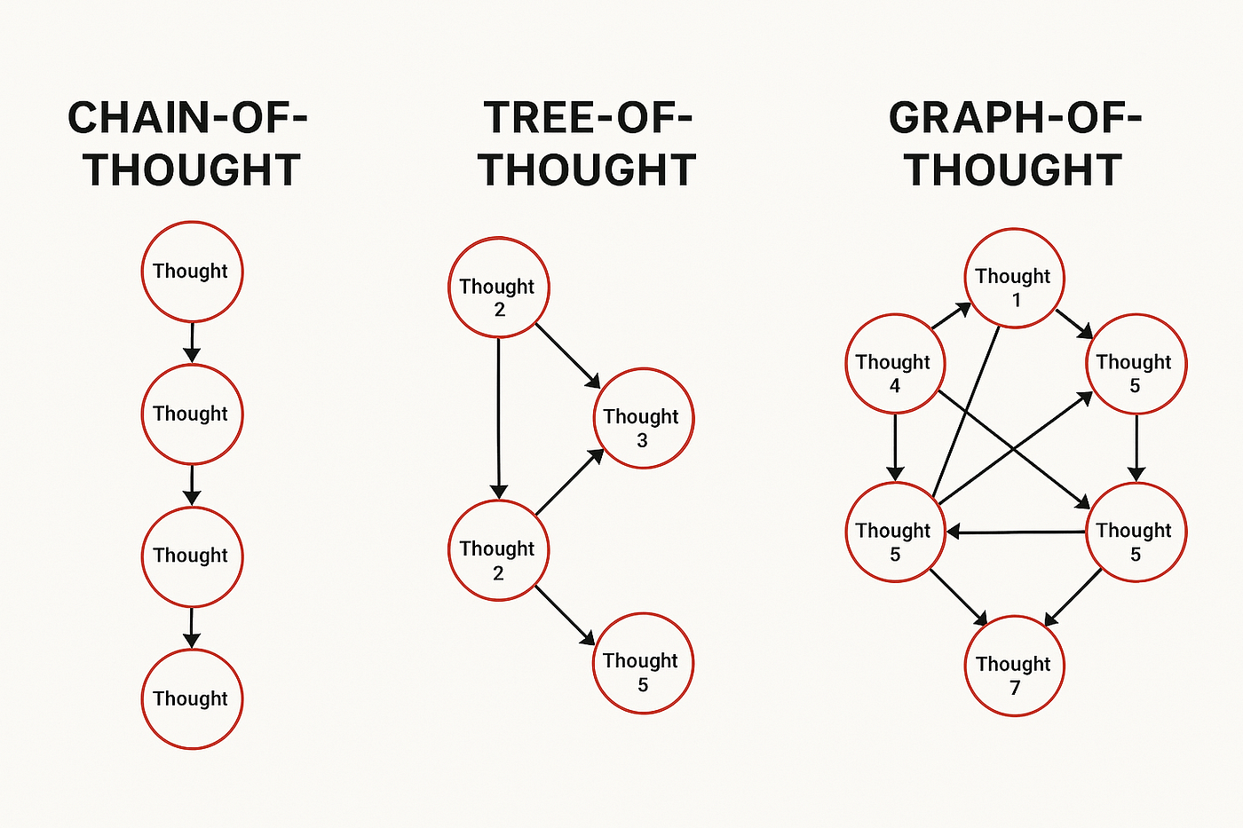
arXiv:2201.11903 [cs.CL]
arXiv:2305.10601 [cs.CL]
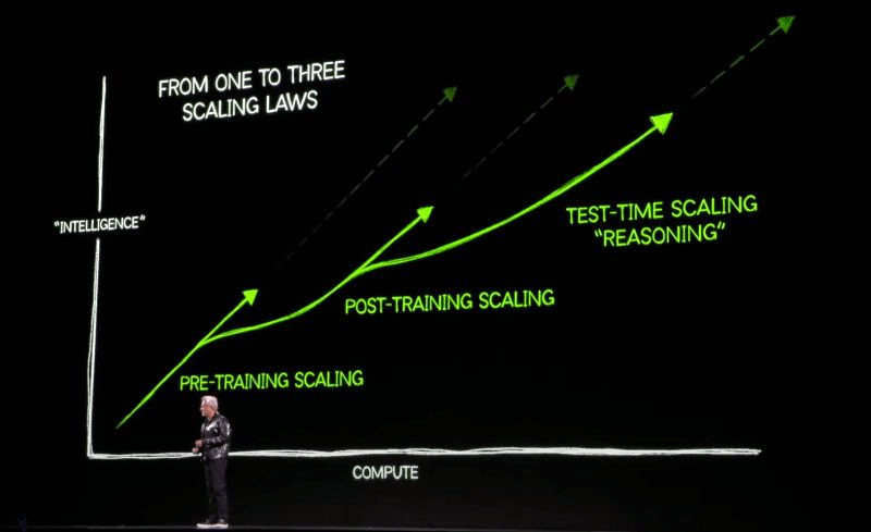
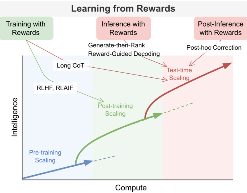
📄 Google DeepMind: "Scaling LLM Test-Time Compute Optimally" (arXiv:2408.03314)
🔗 OpenAI: Learning to Reason with LLMs
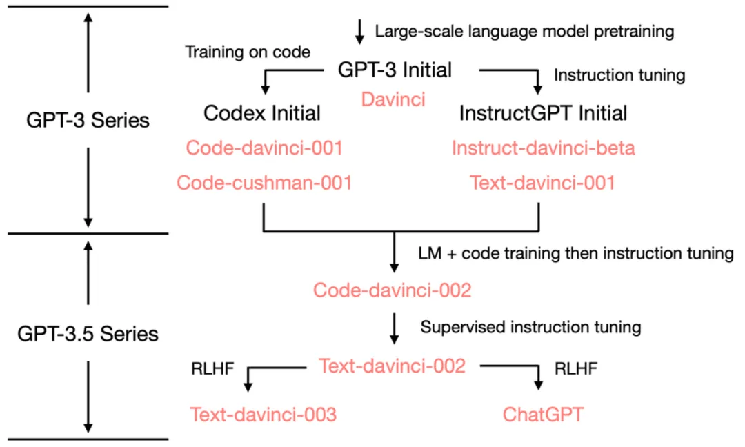
GPT-3.5 series [Source: University of Edinburgh, Allen Institute for AI]
GPT-3 (2020)
ChatGPT (2022)
Magic: Code + Text
究竟是什么让 LLMs 如此强大?
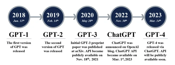
GPT能力的演变
对GPT-3.5能力的仔细审查揭示了其新兴能力的起源:
What are our thoughts on LLMs?
Code! (1/3)
What are our thoughts on LLMs?
究竟是什么让 LLMs 如此颠覆?
Natural Language Programming! (2/3)
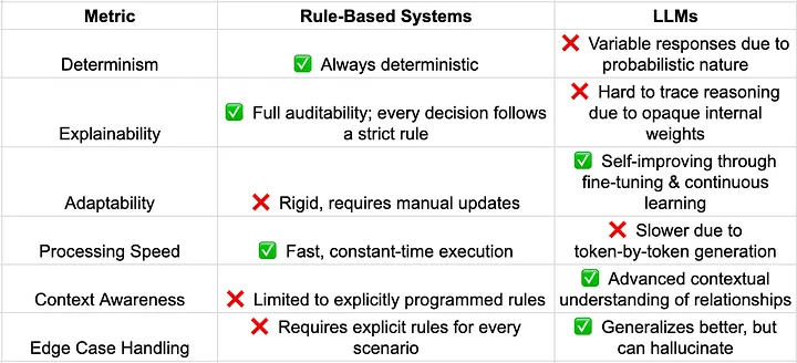
Rule-Based Vs. LLMs: (Source)
What are our thoughts on LLMs?
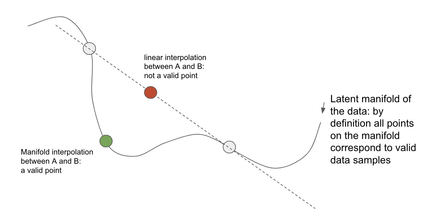
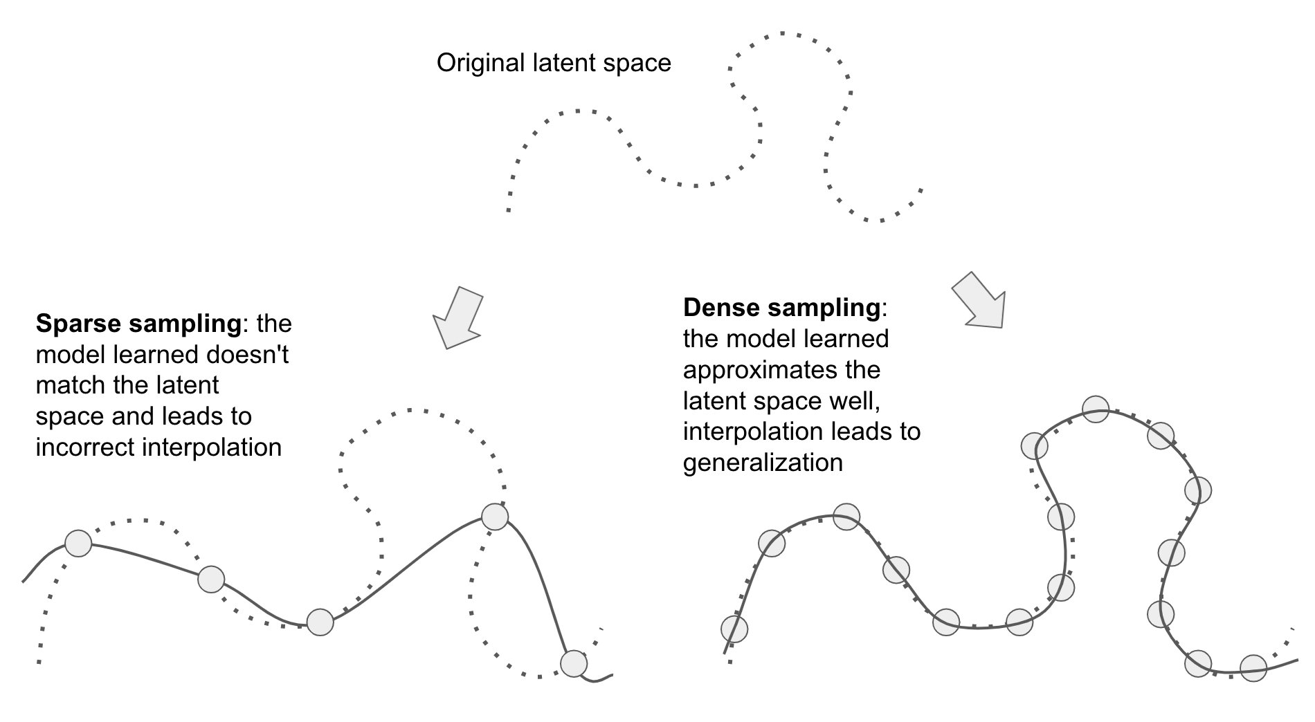
It's Mere Interpolation! (3/3)
Deep Learning is Not As Impressive As you Think, It's Mere Interpolation (Source)
究竟如何解释 AI/LLMs 的原理?
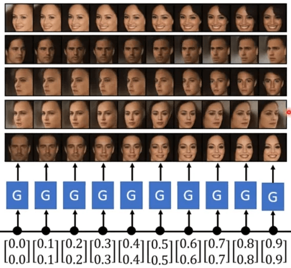
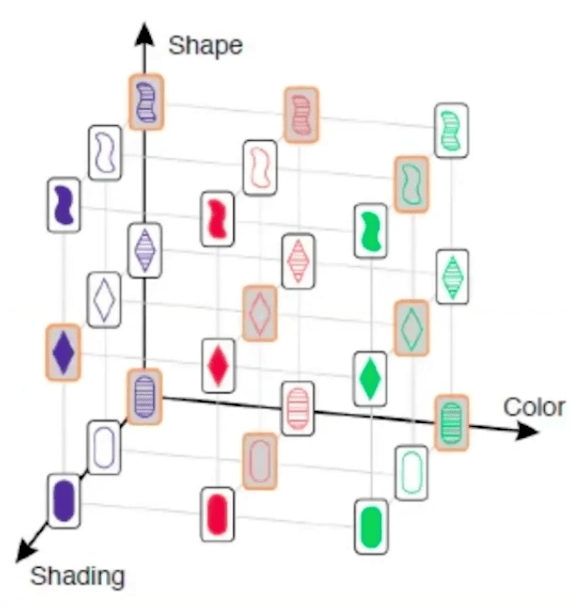
Representation Space Interpolation
The core driving force of AI4Sci largely lies in its “interpolation” generalization capabilities, showcasing its powerful complex modeling abilities.
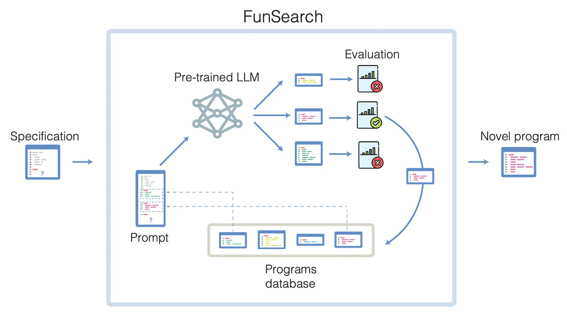
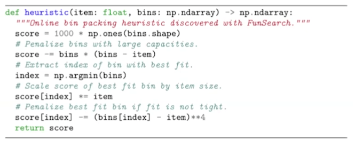
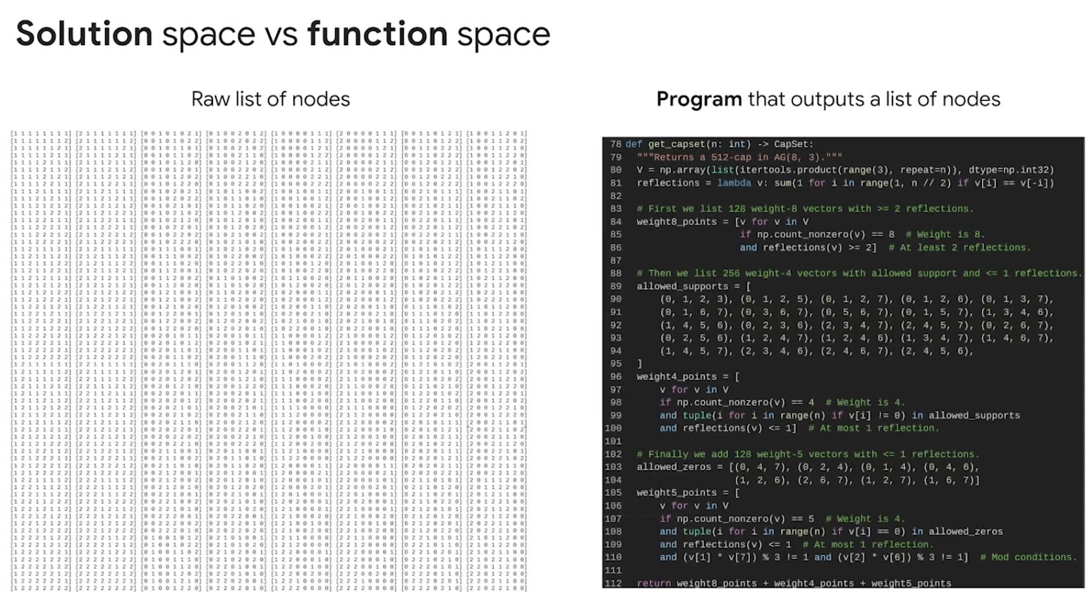
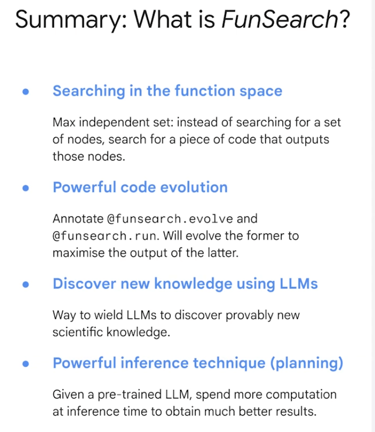
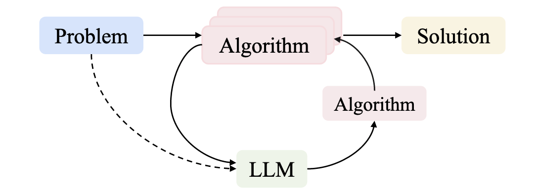
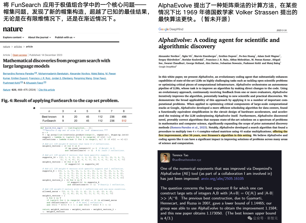
LLM guided search in program space
Illustrative example of bin packing using existing heuristic – Best-fit heuristic (left), and using a heuristic discovered by FunSearch (right).
DeepMind Blog (Source)
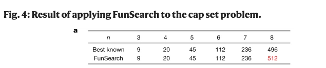
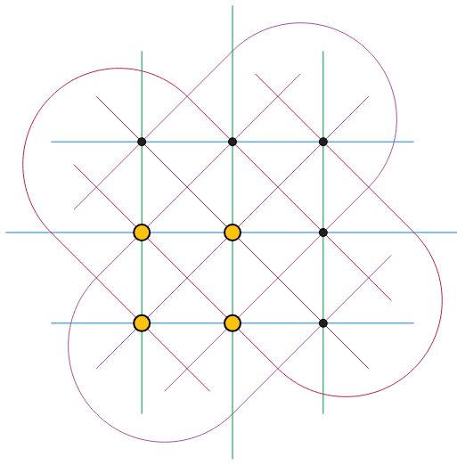
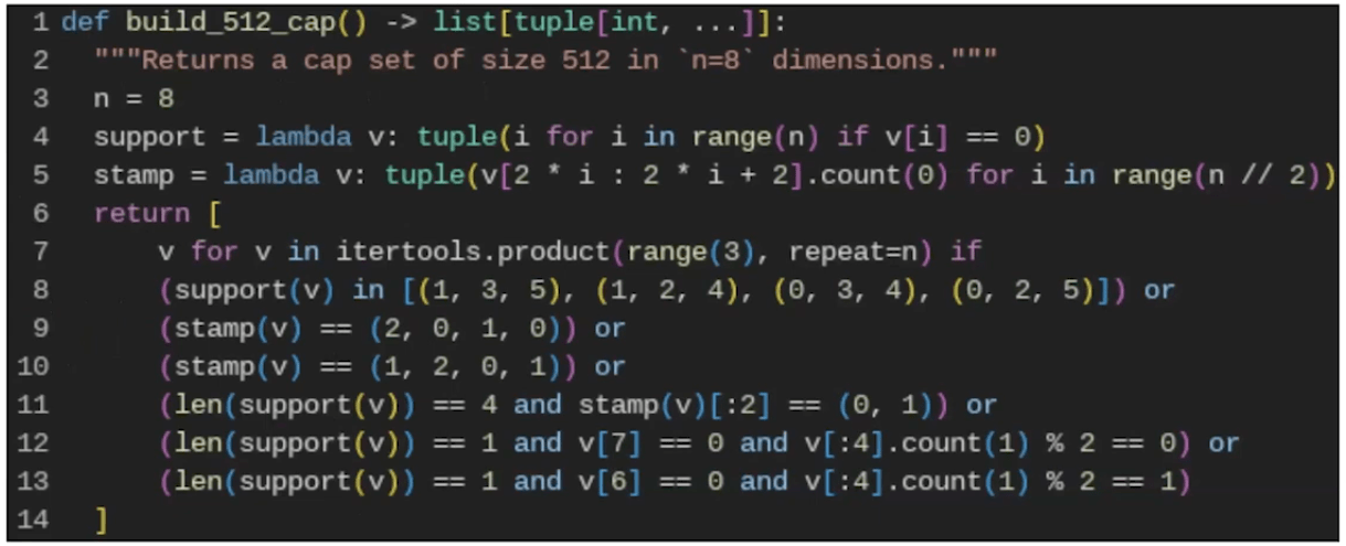
Cap Set Problem
Bin Packing Problem
The largets cap set in N=2 has size 4.
The largest cap set in N=3 has size 9 > \(2^3\)
For N > 6, the size of the largest cap set is unknown.
LLM guided search in program space
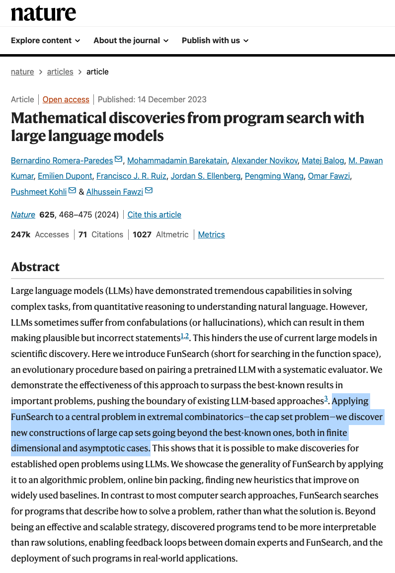
Real-world Case: FunSearch (Nature, 2023)
YouTube (Source)
LLM guided search in program space
YouTube (Source)
Recent research demonstrates that LLMs can solve complex optimization problems through carefully engineered prompts.
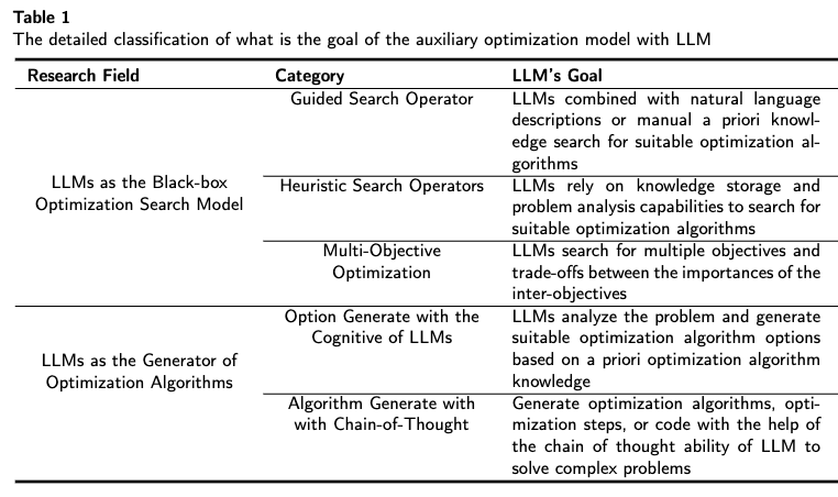
Two Directions of LLM-based Optimization
arXiv:2405.10098 [cs.LG]
arXiv:2410.14716 [cs.LG]
Large Language Models as Designers: LLMs are used to directly create algorithms or specific components,
which are commonly incorporated iteratively to continuously search for better designs.
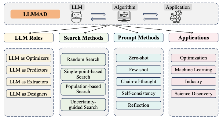
使用LLM实现算法发现解决组合优化问题 (1/3)
arXiv:2402.01145 [cs.NE]
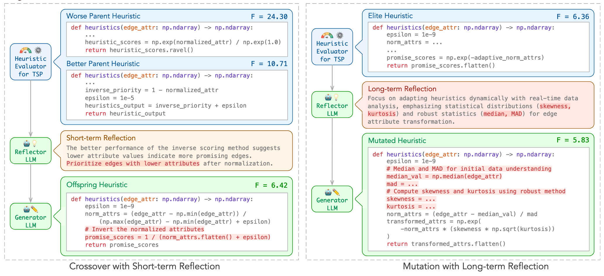
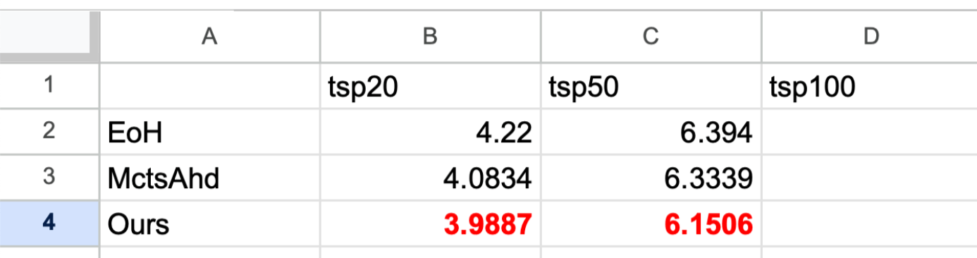
ReEvo
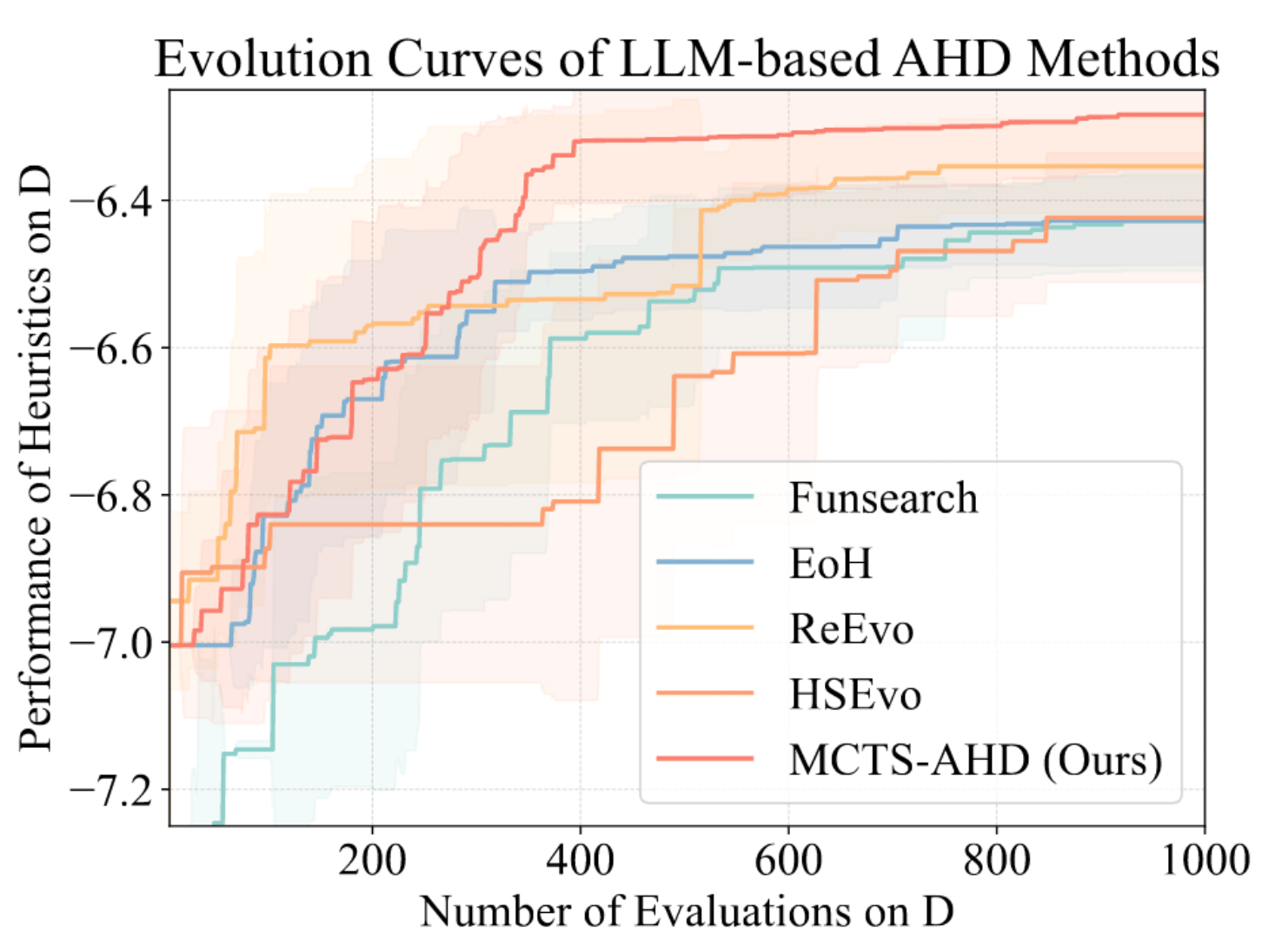
MCTS-AHD
arXiv:2501.08603 [cs.AI]
使用LLM实现算法发现解决组合优化问题 (1/3)
The strict requirements for algorithm discovery
YouTube (Source)
What do we think about LLMs in scientific computing?
(Ours)
使用LLM实现算法发现解决科学计算问题 (2/3)
What do we think about LLMs in gravitational wave science?
使用LLM实现算法发现解决引力波数据处理问题 (3/3)
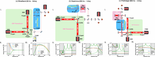
Motivation I: Linear template method using prior data
Motivation II: Black-box data-driven learning methods
Nitz et al., ApJ (2017)
Sci4MLGW@ICERM (June 2025)
For any complex task \(P\) (especially NP-hard problems), Automated Heuristic Design (AHD)
searches for the optimal heuristic \(h^*\) within a heuristic space \(H\):
\(h^*=\underset{h \in H}{\arg \max } g(h) \)
The heuristic space \(H\) contains all feasible algorithmic solutions for task \(P\). Each heuristic \(h \in H\) maps from the set of task inputs \(I_P\) to corresponding solutions \(S_P\):
\(h: I_P \rightarrow S_P\)
Performance measure \(g(\cdot)\) evaluates each heuristic's effectiveness, \(g: H \rightarrow \mathbb{R}\). For minimization problems with objective function \(f: S_P \rightarrow \mathbb{R}\), we estimate performance by evaluating the heuristic instances \({ins}\in D \subseteq I_P\) on dataset \(D\) as follows:
\(g(h)=\mathbb{E}_{\boldsymbol{ins} \in D}[-f(h(\boldsymbol{ins}))]\)
arXiv:2410.14716 [cs.LG]
external_knowledge
(constraint)
arXiv:2410.14716 [cs.LG]
external_knowledge
(constraint)
import numpy as np
import scipy.signal as signal
def pipeline_v1(strain_h1: np.ndarray, strain_l1: np.ndarray, times: np.ndarray) -> tuple[np.ndarray, np.ndarray, np.ndarray]:
    def data_conditioning(strain_h1: np.ndarray, strain_l1: np.ndarray, times: np.ndarray) -> tuple[np.ndarray, np.ndarray, np.ndarray]:
        window_length = 4096
        dt = times[1] - times[0]
        fs = 1.0 / dt

        def whiten_strain(strain):
            strain_zeromean = strain - np.mean(strain)
            freqs, psd = signal.welch(strain_zeromean, fs=fs, nperseg=window_length,
                                       window='hann', noverlap=window_length//2)
            smoothed_psd = np.convolve(psd, np.ones(32) / 32, mode='same')
            smoothed_psd = np.maximum(smoothed_psd, np.finfo(float).tiny)
            white_fft = np.fft.rfft(strain_zeromean) / np.sqrt(np.interp(np.fft.rfftfreq(len(strain_zeromean), d=dt), freqs, smoothed_psd))
            return np.fft.irfft(white_fft)

        whitened_h1 = whiten_strain(strain_h1)
        whitened_l1 = whiten_strain(strain_l1)

        return whitened_h1, whitened_l1, times

    def compute_metric_series(h1_data: np.ndarray, l1_data: np.ndarray, time_series: np.ndarray) -> tuple[np.ndarray, np.ndarray]:
        fs = 1 / (time_series[1] - time_series[0])
        f_h1, t_h1, Sxx_h1 = signal.spectrogram(h1_data, fs=fs, nperseg=256, noverlap=128, mode='magnitude', detrend=False)
        f_l1, t_l1, Sxx_l1 = signal.spectrogram(l1_data, fs=fs, nperseg=256, noverlap=128, mode='magnitude', detrend=False)
        tf_metric = np.mean((Sxx_h1**2 + Sxx_l1**2) / 2, axis=0)
        gps_mid_time = time_series[0] + (time_series[-1] - time_series[0]) / 2
        metric_times = gps_mid_time + (t_h1 - t_h1[-1] / 2)

        return tf_metric, metric_times

    def calculate_statistics(tf_metric, t_h1):
        background_level = np.median(tf_metric)
        peaks, _ = signal.find_peaks(tf_metric, height=background_level * 1.0, distance=2, prominence=background_level * 0.3)
        peak_times = t_h1[peaks]
        peak_heights = tf_metric[peaks]
        peak_deltat = np.full(len(peak_times), 10.0)  # Fixed uncertainty value
        return peak_times, peak_heights, peak_deltat

    whitened_h1, whitened_l1, data_times = data_conditioning(strain_h1, strain_l1, times)
    tf_metric, metric_times = compute_metric_series(whitened_h1, whitened_l1, data_times)
    peak_times, peak_heights, peak_deltat = calculate_statistics(tf_metric, metric_times)

    return peak_times, peak_heights, peak_deltat
Input: H1 and L1 detector strains, time array | Output: Event times, significance values, and time uncertainties
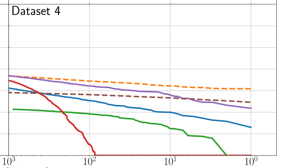
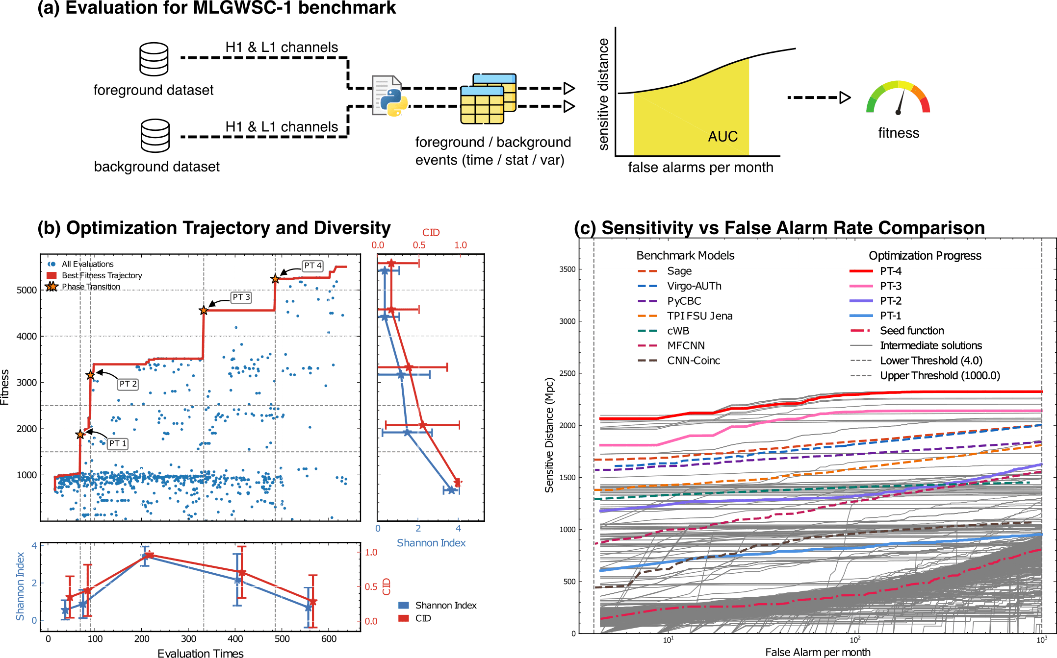
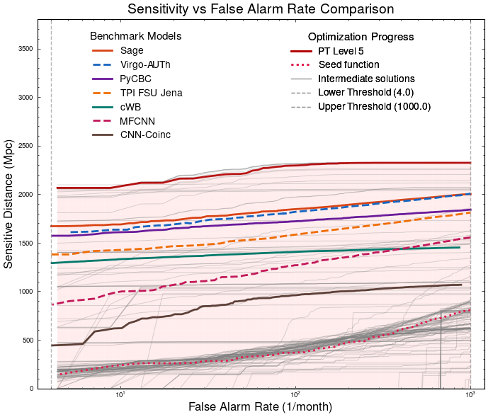
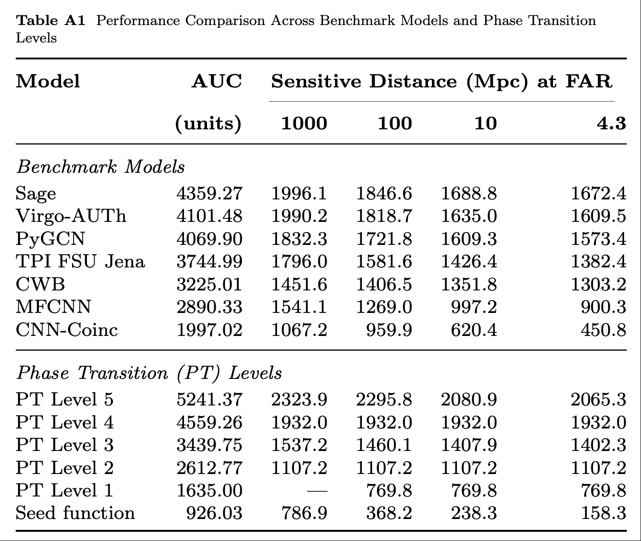
Optimization Target: Maximizing Area Under Curve (AUC) in the 1-1000Hz false alarms per-year range, balancing detection sensitivity and false alarm rates across algorithm generations
MLGWSC-1 benchmark
Problem: Pipeline Workflow
arXiv:2410.14716 [cs.LG]
external_knowledge
(constraint)
Optimization Target: Maximizing Area Under Curve (AUC) in the 1-1000Hz false alarms per-year range, balancing detection sensitivity and false alarm rates across algorithm generations
MLGWSC-1 benchmark
Evaluation for MLGWSC-1 benchmark
Strategies for Adapting Gravitational Wave Detection for Algorithmic Discovery
arXiv:2410.14716 [cs.LG]
external_knowledge
(constraint)
You are an expert in gravitational wave signal detection algorithms. Your task is to design heuristics that can effectively solve optimization problems.

{prompt_task}

I have analyzed two algorithms and provided a reflection on their differences.

[Worse code]
{worse_code}

[Better code]
{better_code}

[Reflection]
{reflection}

{external_knowledge}

Based on this reflection, please write an improved algorithm according to the reflection.
First, describe the design idea and main steps of your algorithm in one sentence. The description must be inside a brace outside the code implementation. Next, implement it in Python as a function named '{func_name}'.
This function should accept {input_count} input(s): {joined_inputs}. The function should return {output_count} output(s): {joined_outputs}.
{inout_inf} {other_inf}

Do not give additional explanations.
One Prompt Template for MLGWSC1 Algorithm Synthesis
Strategies for Adapting Gravitational Wave Detection for Algorithmic Discovery
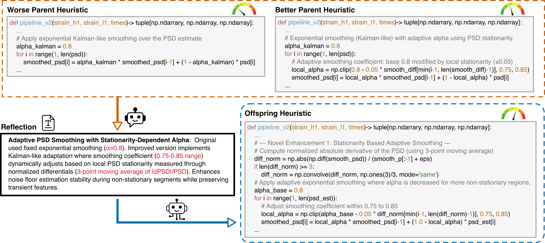
Prompt Structure for Algorithm Evolution
This template guides the LLM to generate optimized gravitational wave detection algorithms by learning from comparative examples ("Crossover").
Key Components:
hewang@ucas.ac.cn
LLM-Informed Evo-MCTS for AAD
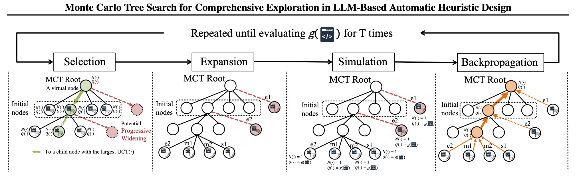
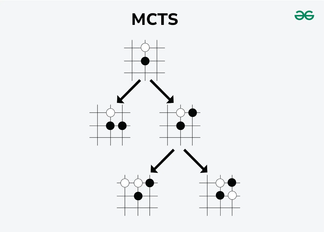
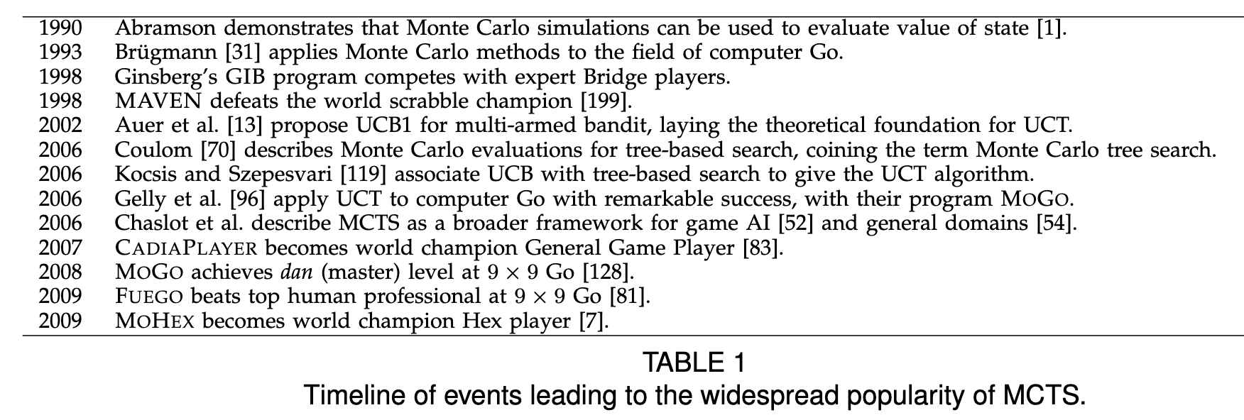
蒙特卡洛树搜索 (MCTS)
hewang@ucas.ac.cn
LLM-Informed Evo-MCTS for AAD
蒙特卡洛树搜索 (MCTS)
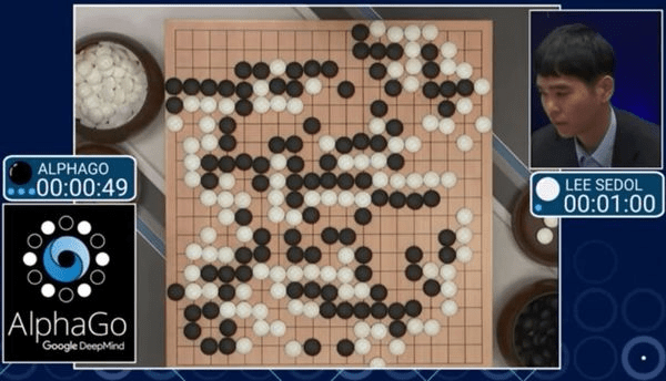
Casse1: Go Game
Case 2: OpenAI Strawberry (o1)
o1 的发布,标志着推理时间扩展(inference-time scaling)范式正式应用于生产环境。正如Sutton在《The Bitter Lesson》中指出,只有学习和搜索两种技术能随计算能力无限扩展。自此开始重点转向搜索了。
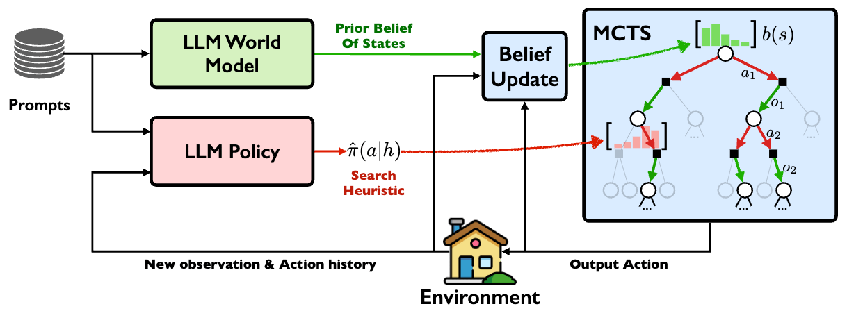
arXiv:2305.14078 [cs.RO]
Browne et al. (2012)
arXiv:2305.14078 [cs.RO]
蒙特卡洛树搜索(MCTS)结合随机模拟与树搜索优化决策,(一直)都是现代博弈程序(如AlphaGo)的核心技术。
hewang@ucas.ac.cn
LLM-Informed Evo-MCTS for AAD
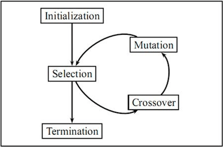
进化演化 (EA)
external_knowledge
(constraint)
hewang@ucas.ac.cn
LLM-Informed Evo-MCTS for AAD
LLM-Driven Algorithmic Evolution Through Reflective Code Synthesis.
external_knowledge
(constraint)
hewang@ucas.ac.cn
Automated exploration of algorithm parameter space
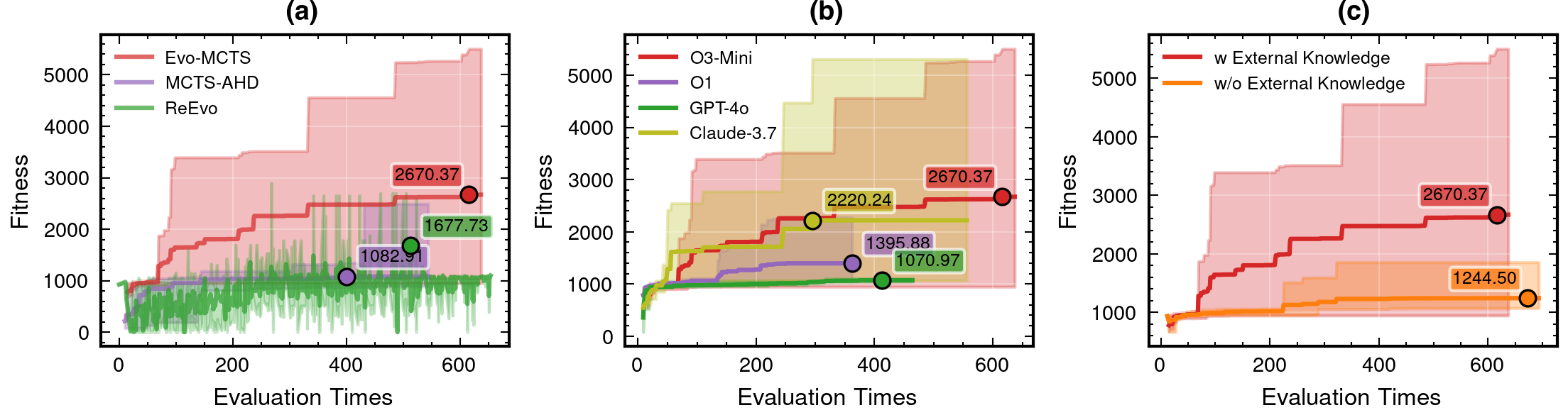
Benchmarking against state-of-the-art methods
external_knowledge
(constraint)
hewang@ucas.ac.cn
Automated exploration of algorithm parameter space
Benchmarking against state-of-the-art methods
PyCBC (linear-core)
cWB (nonlinear-core)
Simple filters (non-linear)
CNN-like (highly non-linear)
20.2%
23.4%
external_knowledge
(constraint)
hewang@ucas.ac.cn
PyCBC (linear-core)
cWB (nonlinear-core)
Simple filters (non-linear)
CNN-like (highly non-linear)
Automated exploration of algorithm parameter space
Benchmarking against state-of-the-art methods
20.2%
23.4%
external_knowledge
(constraint)
hewang@ucas.ac.cn
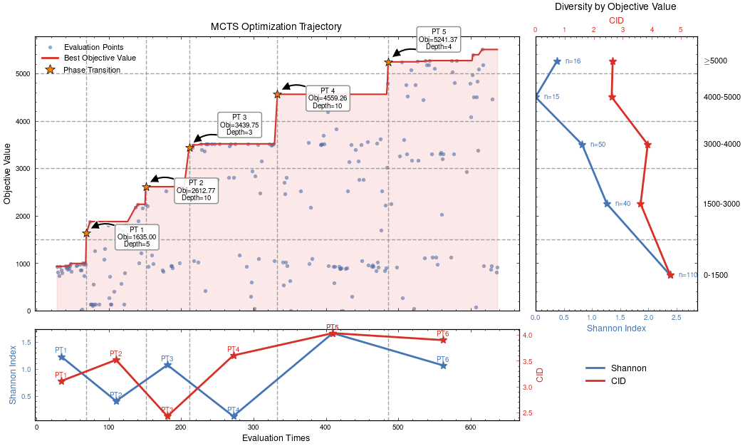
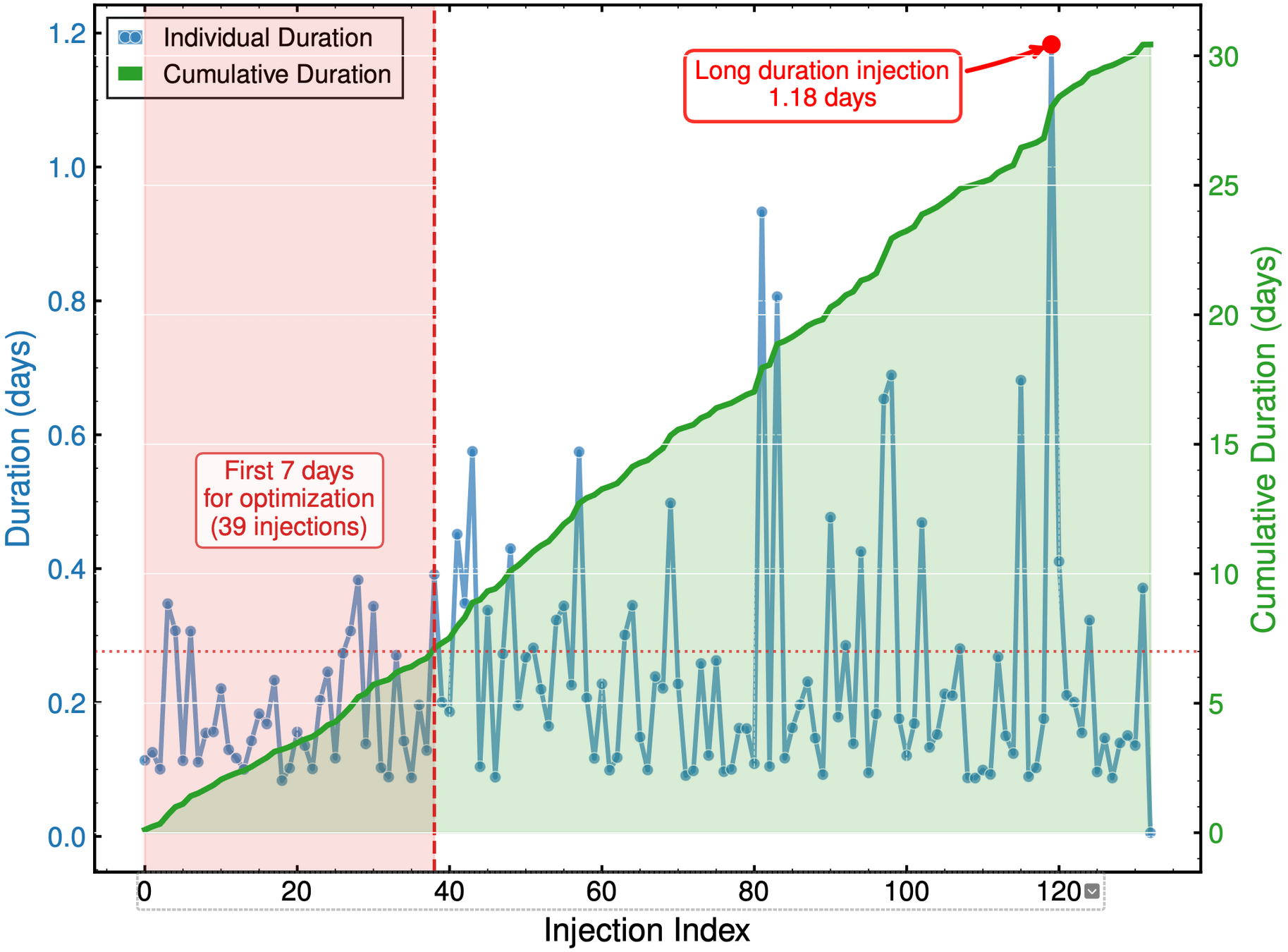
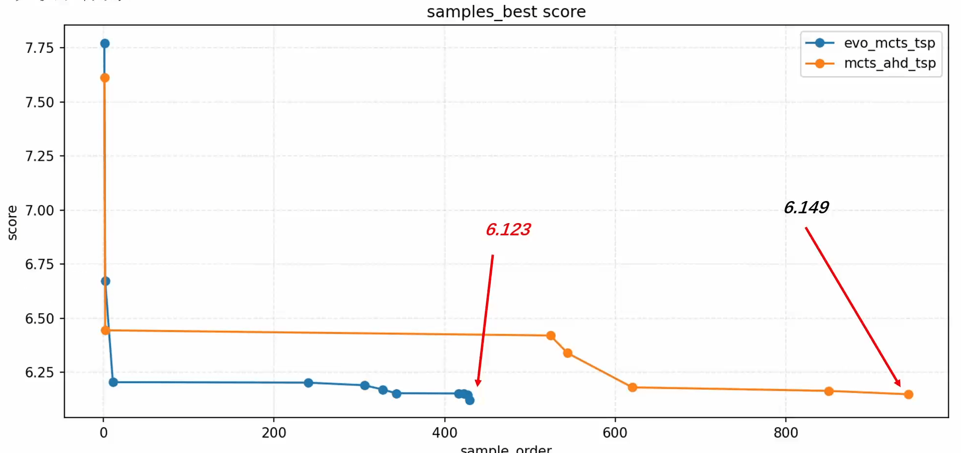
Optimization Progress & Algorithm Diversity
Interpretable Gravitational Wave Data Analysis with DL and LLMs
Diversity metrics:
Diversity in Evolutionary Computation
Population encoding:
hewang@ucas.ac.cn
Automated exploration of algorithm parameter space
Benchmarking against state-of-the-art methods
PyCBC (linear-core)
cWB (nonlinear-core)
Simple filters (non-linear)
CNN-like (highly non-linear)
20.2%
23.4%
hewang@ucas.ac.cn
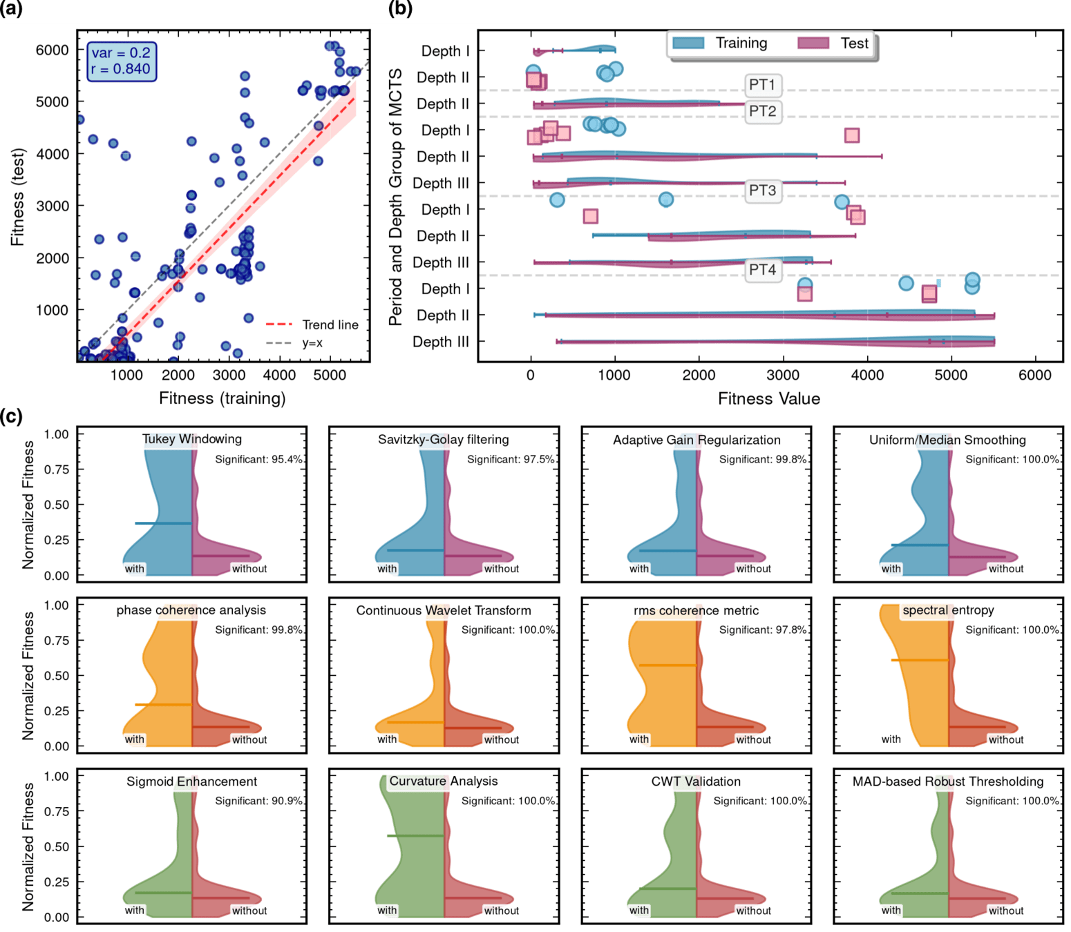
Algorithmic Component Impact Analysis.
AAD for GW detection Guided by LLM-informed Evo-MCTS
import numpy as np
import scipy.signal as signal
from scipy.signal.windows import tukey
from scipy.signal import savgol_filter

def pipeline_v2(strain_h1: np.ndarray, strain_l1: np.ndarray, times: np.ndarray) -> tuple[np.ndarray, np.ndarray, np.ndarray]:
    """
    The pipeline function processes gravitational wave data from the H1 and L1 detectors to identify potential gravitational wave signals.
    It takes strain_h1 and strain_l1 numpy arrays containing detector data, and times array with corresponding time points.
    The function returns a tuple of three numpy arrays: peak_times containing GPS times of identified events,
    peak_heights with significance values of each peak, and peak_deltat showing time window uncertainty for each peak.
    """
    eps = np.finfo(float).tiny
    dt = times[1] - times[0]
    fs = 1.0 / dt
    # Base spectrogram parameters
    base_nperseg = 256
    base_noverlap = base_nperseg // 2
    medfilt_kernel = 101       # odd kernel size for robust detrending
    uncertainty_window = 5     # half-window for local timing uncertainty

    # -------------------- Stage 1: Robust Baseline Detrending --------------------
    # Remove long-term trends using a median filter for each channel.
    detrended_h1 = strain_h1 - signal.medfilt(strain_h1, kernel_size=medfilt_kernel)
    detrended_l1 = strain_l1 - signal.medfilt(strain_l1, kernel_size=medfilt_kernel)

    # -------------------- Stage 2: Adaptive Whitening with Enhanced PSD Smoothing --------------------
    def adaptive_whitening(strain: np.ndarray) -> np.ndarray:
        # Center the signal.
        centered = strain - np.mean(strain)
        n_samples = len(centered)
        # Adaptive window length: between 5 and 30 seconds
        win_length_sec = np.clip(n_samples / fs / 20, 5, 30)
        nperseg_adapt = int(win_length_sec * fs)
        nperseg_adapt = max(10, min(nperseg_adapt, n_samples))

        # Create a Tukey window with 75% overlap.
        tukey_alpha = 0.25
        win = tukey(nperseg_adapt, alpha=tukey_alpha)
        noverlap_adapt = int(nperseg_adapt * 0.75)
        if noverlap_adapt >= nperseg_adapt:
            noverlap_adapt = nperseg_adapt - 1

        # Estimate the power spectral density (PSD) using Welch's method.
        freqs, psd = signal.welch(centered, fs=fs, nperseg=nperseg_adapt,
                                  noverlap=noverlap_adapt, window=win, detrend='constant')
        psd = np.maximum(psd, eps)

        # Compute relative differences for PSD stationarity measure.
        diff_arr = np.abs(np.diff(psd)) / (psd[:-1] + eps)
        # Smooth the derivative with a moving average.
        if len(diff_arr) >= 3:
            smooth_diff = np.convolve(diff_arr, np.ones(3)/3, mode='same')
        else:
            smooth_diff = diff_arr

        # Exponential smoothing (Kalman-like) with adaptive alpha using PSD stationarity.
        smoothed_psd = np.copy(psd)
        for i in range(1, len(psd)):
            # Adaptive smoothing coefficient: base 0.8 modified by local stationarity (±0.05)
            local_alpha = np.clip(0.8 - 0.05 * smooth_diff[min(i-1, len(smooth_diff)-1)], 0.75, 0.85)
            smoothed_psd[i] = local_alpha * smoothed_psd[i-1] + (1 - local_alpha) * psd[i]

        # Compute Tikhonov regularization gain based on deviation from median PSD.
        noise_baseline = np.median(smoothed_psd)
        raw_gain = (smoothed_psd / (noise_baseline + eps)) - 1.0

        # Compute a causal-like gradient using the Savitzky-Golay filter.
        win_len = 11 if len(smoothed_psd) >= 11 else ((len(smoothed_psd)//2)*2+1)
        polyorder = 2 if win_len > 2 else 1
        delta_freq = np.mean(np.diff(freqs))
        grad_psd = savgol_filter(smoothed_psd, win_len, polyorder, deriv=1, delta=delta_freq, mode='interp')

        # Nonlinear scaling via sigmoid to enhance gradient differences.
        sigmoid = lambda x: 1.0 / (1.0 + np.exp(-x))
        scaling_factor = 1.0 + 2.0 * sigmoid(np.abs(grad_psd) / (np.median(smoothed_psd) + eps))

        # Compute adaptive gain factors with nonlinear scaling.
        gain = 1.0 - np.exp(-0.5 * scaling_factor * raw_gain)
        gain = np.clip(gain, -8.0, 8.0)

        # FFT-based whitening: interpolate gain and PSD onto FFT frequency bins.
        signal_fft = np.fft.rfft(centered)
        freq_bins = np.fft.rfftfreq(n_samples, d=dt)
        interp_gain = np.interp(freq_bins, freqs, gain, left=gain[0], right=gain[-1])
        interp_psd = np.interp(freq_bins, freqs, smoothed_psd, left=smoothed_psd[0], right=smoothed_psd[-1])
        denom = np.sqrt(interp_psd) * (np.abs(interp_gain) + eps)
        denom = np.maximum(denom, eps)
        white_fft = signal_fft / denom
        whitened = np.fft.irfft(white_fft, n=n_samples)
        return whitened

    # Whiten H1 and L1 channels using the adapted method.
    white_h1 = adaptive_whitening(detrended_h1)
    white_l1 = adaptive_whitening(detrended_l1)

    # -------------------- Stage 3: Coherent Time-Frequency Metric with Frequency-Conditioned Regularization --------------------
    def compute_coherent_metric(w1: np.ndarray, w2: np.ndarray) -> tuple[np.ndarray, np.ndarray]:
        # Compute complex spectrograms preserving phase information.
        f1, t_spec, Sxx1 = signal.spectrogram(w1, fs=fs, nperseg=base_nperseg,
                                              noverlap=base_noverlap, mode='complex', detrend=False)
        f2, t_spec2, Sxx2 = signal.spectrogram(w2, fs=fs, nperseg=base_nperseg,
                                               noverlap=base_noverlap, mode='complex', detrend=False)
        # Ensure common time axis length.
        common_len = min(len(t_spec), len(t_spec2))
        t_spec = t_spec[:common_len]
        Sxx1 = Sxx1[:, :common_len]
        Sxx2 = Sxx2[:, :common_len]

        # Compute phase differences and coherence between detectors.
        phase_diff = np.angle(Sxx1) - np.angle(Sxx2)
        phase_coherence = np.abs(np.cos(phase_diff))

        # Estimate median PSD per frequency bin from the spectrograms.
        psd1 = np.median(np.abs(Sxx1)**2, axis=1)
        psd2 = np.median(np.abs(Sxx2)**2, axis=1)

        # Frequency-conditioned regularization gain (reflection-guided).
        lambda_f = 0.5 * ((np.median(psd1) / (psd1 + eps)) + (np.median(psd2) / (psd2 + eps)))
        lambda_f = np.clip(lambda_f, 1e-4, 1e-2)
        # Regularization denominator integrating detector PSDs and lambda.
        reg_denom = (psd1[:, None] + psd2[:, None] + lambda_f[:, None] + eps)

        # Weighted phase coherence that balances phase alignment with noise levels.
        weighted_comp = phase_coherence / reg_denom

        # Compute axial (frequency) second derivatives as curvature estimates.
        d2_coh = np.gradient(np.gradient(phase_coherence, axis=0), axis=0)
        avg_curvature = np.mean(np.abs(d2_coh), axis=0)

        # Nonlinear activation boost using tanh for regions of high curvature.
        nonlinear_boost = np.tanh(5 * avg_curvature)
        linear_boost = 1.0 + 0.1 * avg_curvature

        # Cross-detector synergy: weight derived from global median consistency.
        novel_weight = np.mean((np.median(psd1) + np.median(psd2)) / (psd1[:, None] + psd2[:, None] + eps), axis=0)

        # Integrated time-frequency metric combining all enhancements.
        tf_metric = np.sum(weighted_comp * linear_boost * (1.0 + nonlinear_boost), axis=0) * novel_weight

        # Adjust the spectrogram time axis to account for window delay.
        metric_times = t_spec + times[0] + (base_nperseg / 2) / fs
        return tf_metric, metric_times

    tf_metric, metric_times = compute_coherent_metric(white_h1, white_l1)

    # -------------------- Stage 4: Multi-Resolution Thresholding with Octave-Spaced Dyadic Wavelet Validation --------------------
    def multi_resolution_thresholding(metric: np.ndarray, times_arr: np.ndarray) -> tuple[np.ndarray, np.ndarray, np.ndarray]:
        # Robust background estimation with median and MAD.
        bg_level = np.median(metric)
        mad_val = np.median(np.abs(metric - bg_level))
        robust_std = 1.4826 * mad_val
        threshold = bg_level + 1.5 * robust_std

        # Identify candidate peaks using prominence and minimum distance criteria.
        peaks, _ = signal.find_peaks(metric, height=threshold, distance=2, prominence=0.8 * robust_std)
        if peaks.size == 0:
            return np.array([]), np.array([]), np.array([])

        # Local uncertainty estimation using a Gaussian-weighted convolution.
        win_range = np.arange(-uncertainty_window, uncertainty_window + 1)
        sigma = uncertainty_window / 2.5
        gauss_kernel = np.exp(-0.5 * (win_range / sigma) ** 2)
        gauss_kernel /= np.sum(gauss_kernel)
        weighted_mean = np.convolve(metric, gauss_kernel, mode='same')
        weighted_sq = np.convolve(metric ** 2, gauss_kernel, mode='same')
        variances = np.maximum(weighted_sq - weighted_mean ** 2, 0.0)
        uncertainties = np.sqrt(variances)
        uncertainties = np.maximum(uncertainties, 0.01)

        valid_times = []
        valid_heights = []
        valid_uncerts = []
        n_metric = len(metric)

        # Compute a simple second derivative for local curvature checking.
        if n_metric > 2:
            second_deriv = np.diff(metric, n=2)
            second_deriv = np.pad(second_deriv, (1, 1), mode='edge')
        else:
            second_deriv = np.zeros_like(metric)

        # Use octave-spaced scales (dyadic wavelet validation) to validate peak significance.
        widths = np.arange(1, 9)  # approximate scales 1 to 8
        for peak in peaks:
            # Skip peaks lacking sufficient negative curvature.
            if second_deriv[peak] > -0.1 * robust_std:
                continue
            local_start = max(0, peak - uncertainty_window)
            local_end = min(n_metric, peak + uncertainty_window + 1)
            local_segment = metric[local_start:local_end]
            if len(local_segment) < 3:
                continue
            try:
                cwt_coeff = signal.cwt(local_segment, signal.ricker, widths)
            except Exception:
                continue
            max_coeff = np.max(np.abs(cwt_coeff))
            # Threshold for validating the candidate using local MAD.
            cwt_thresh = mad_val * np.sqrt(2 * np.log(len(local_segment) + eps))
            if max_coeff >= cwt_thresh:
                valid_times.append(times_arr[peak])
                valid_heights.append(metric[peak])
                valid_uncerts.append(uncertainties[peak])

        if len(valid_times) == 0:
            return np.array([]), np.array([]), np.array([])
        return np.array(valid_times), np.array(valid_heights), np.array(valid_uncerts)

    peak_times, peak_heights, peak_deltat = multi_resolution_thresholding(tf_metric, metric_times)
return peak_times, peak_heights, peak_deltatPT Level 5
import numpy as np
import scipy.signal as signal
from scipy.signal.windows import tukey
from scipy.signal import savgol_filter

def pipeline_v2(strain_h1: np.ndarray, strain_l1: np.ndarray, times: np.ndarray) -> tuple[np.ndarray, np.ndarray, np.ndarray]:
    """
    The pipeline function processes gravitational wave data from the H1 and L1 detectors to identify potential gravitational wave signals.
    It takes strain_h1 and strain_l1 numpy arrays containing detector data, and times array with corresponding time points.
    The function returns a tuple of three numpy arrays: peak_times containing GPS times of identified events,
    peak_heights with significance values of each peak, and peak_deltat showing time window uncertainty for each peak.
    """
    eps = np.finfo(float).tiny
    dt = times[1] - times[0]
    fs = 1.0 / dt
    # Base spectrogram parameters
    base_nperseg = 256
    base_noverlap = base_nperseg // 2
    medfilt_kernel = 101       # odd kernel size for robust detrending
    uncertainty_window = 5     # half-window for local timing uncertainty

    # -------------------- Stage 1: Robust Baseline Detrending --------------------
    # Remove long-term trends using a median filter for each channel.
    detrended_h1 = strain_h1 - signal.medfilt(strain_h1, kernel_size=medfilt_kernel)
    detrended_l1 = strain_l1 - signal.medfilt(strain_l1, kernel_size=medfilt_kernel)

    # -------------------- Stage 2: Adaptive Whitening with Enhanced PSD Smoothing --------------------
    def adaptive_whitening(strain: np.ndarray) -> np.ndarray:
        # Center the signal.
        centered = strain - np.mean(strain)
        n_samples = len(centered)
        # Adaptive window length: between 5 and 30 seconds
        win_length_sec = np.clip(n_samples / fs / 20, 5, 30)
        nperseg_adapt = int(win_length_sec * fs)
        nperseg_adapt = max(10, min(nperseg_adapt, n_samples))

        # Create a Tukey window with 75% overlap.
        tukey_alpha = 0.25
        win = tukey(nperseg_adapt, alpha=tukey_alpha)
        noverlap_adapt = int(nperseg_adapt * 0.75)
        if noverlap_adapt >= nperseg_adapt:
            noverlap_adapt = nperseg_adapt - 1

        # Estimate the power spectral density (PSD) using Welch's method.
        freqs, psd = signal.welch(centered, fs=fs, nperseg=nperseg_adapt,
                                  noverlap=noverlap_adapt, window=win, detrend='constant')
        psd = np.maximum(psd, eps)

        # Compute relative differences for PSD stationarity measure.
        diff_arr = np.abs(np.diff(psd)) / (psd[:-1] + eps)
        # Smooth the derivative with a moving average.
        if len(diff_arr) >= 3:
            smooth_diff = np.convolve(diff_arr, np.ones(3)/3, mode='same')
        else:
            smooth_diff = diff_arr

        # Exponential smoothing (Kalman-like) with adaptive alpha using PSD stationarity.
        smoothed_psd = np.copy(psd)
        for i in range(1, len(psd)):
            # Adaptive smoothing coefficient: base 0.8 modified by local stationarity (±0.05)
            local_alpha = np.clip(0.8 - 0.05 * smooth_diff[min(i-1, len(smooth_diff)-1)], 0.75, 0.85)
            smoothed_psd[i] = local_alpha * smoothed_psd[i-1] + (1 - local_alpha) * psd[i]

        # Compute Tikhonov regularization gain based on deviation from median PSD.
        noise_baseline = np.median(smoothed_psd)
        raw_gain = (smoothed_psd / (noise_baseline + eps)) - 1.0

        # Compute a causal-like gradient using the Savitzky-Golay filter.
        win_len = 11 if len(smoothed_psd) >= 11 else ((len(smoothed_psd)//2)*2+1)
        polyorder = 2 if win_len > 2 else 1
        delta_freq = np.mean(np.diff(freqs))
        grad_psd = savgol_filter(smoothed_psd, win_len, polyorder, deriv=1, delta=delta_freq, mode='interp')

        # Nonlinear scaling via sigmoid to enhance gradient differences.
        sigmoid = lambda x: 1.0 / (1.0 + np.exp(-x))
        scaling_factor = 1.0 + 2.0 * sigmoid(np.abs(grad_psd) / (np.median(smoothed_psd) + eps))

        # Compute adaptive gain factors with nonlinear scaling.
        gain = 1.0 - np.exp(-0.5 * scaling_factor * raw_gain)
        gain = np.clip(gain, -8.0, 8.0)

        # FFT-based whitening: interpolate gain and PSD onto FFT frequency bins.
        signal_fft = np.fft.rfft(centered)
        freq_bins = np.fft.rfftfreq(n_samples, d=dt)
        interp_gain = np.interp(freq_bins, freqs, gain, left=gain[0], right=gain[-1])
        interp_psd = np.interp(freq_bins, freqs, smoothed_psd, left=smoothed_psd[0], right=smoothed_psd[-1])
        denom = np.sqrt(interp_psd) * (np.abs(interp_gain) + eps)
        denom = np.maximum(denom, eps)
        white_fft = signal_fft / denom
        whitened = np.fft.irfft(white_fft, n=n_samples)
        return whitened

    # Whiten H1 and L1 channels using the adapted method.
    white_h1 = adaptive_whitening(detrended_h1)
    white_l1 = adaptive_whitening(detrended_l1)

    # -------------------- Stage 3: Coherent Time-Frequency Metric with Frequency-Conditioned Regularization --------------------
    def compute_coherent_metric(w1: np.ndarray, w2: np.ndarray) -> tuple[np.ndarray, np.ndarray]:
        # Compute complex spectrograms preserving phase information.
        f1, t_spec, Sxx1 = signal.spectrogram(w1, fs=fs, nperseg=base_nperseg,
                                              noverlap=base_noverlap, mode='complex', detrend=False)
        f2, t_spec2, Sxx2 = signal.spectrogram(w2, fs=fs, nperseg=base_nperseg,
                                               noverlap=base_noverlap, mode='complex', detrend=False)
        # Ensure common time axis length.
        common_len = min(len(t_spec), len(t_spec2))
        t_spec = t_spec[:common_len]
        Sxx1 = Sxx1[:, :common_len]
        Sxx2 = Sxx2[:, :common_len]

        # Compute phase differences and coherence between detectors.
        phase_diff = np.angle(Sxx1) - np.angle(Sxx2)
        phase_coherence = np.abs(np.cos(phase_diff))

        # Estimate median PSD per frequency bin from the spectrograms.
        psd1 = np.median(np.abs(Sxx1)**2, axis=1)
        psd2 = np.median(np.abs(Sxx2)**2, axis=1)

        # Frequency-conditioned regularization gain (reflection-guided).
        lambda_f = 0.5 * ((np.median(psd1) / (psd1 + eps)) + (np.median(psd2) / (psd2 + eps)))
        lambda_f = np.clip(lambda_f, 1e-4, 1e-2)
        # Regularization denominator integrating detector PSDs and lambda.
        reg_denom = (psd1[:, None] + psd2[:, None] + lambda_f[:, None] + eps)

        # Weighted phase coherence that balances phase alignment with noise levels.
        weighted_comp = phase_coherence / reg_denom

        # Compute axial (frequency) second derivatives as curvature estimates.
        d2_coh = np.gradient(np.gradient(phase_coherence, axis=0), axis=0)
        avg_curvature = np.mean(np.abs(d2_coh), axis=0)

        # Nonlinear activation boost using tanh for regions of high curvature.
        nonlinear_boost = np.tanh(5 * avg_curvature)
        linear_boost = 1.0 + 0.1 * avg_curvature

        # Cross-detector synergy: weight derived from global median consistency.
        novel_weight = np.mean((np.median(psd1) + np.median(psd2)) / (psd1[:, None] + psd2[:, None] + eps), axis=0)

        # Integrated time-frequency metric combining all enhancements.
        tf_metric = np.sum(weighted_comp * linear_boost * (1.0 + nonlinear_boost), axis=0) * novel_weight

        # Adjust the spectrogram time axis to account for window delay.
        metric_times = t_spec + times[0] + (base_nperseg / 2) / fs
        return tf_metric, metric_times

    tf_metric, metric_times = compute_coherent_metric(white_h1, white_l1)

    # -------------------- Stage 4: Multi-Resolution Thresholding with Octave-Spaced Dyadic Wavelet Validation --------------------
    def multi_resolution_thresholding(metric: np.ndarray, times_arr: np.ndarray) -> tuple[np.ndarray, np.ndarray, np.ndarray]:
        # Robust background estimation with median and MAD.
        bg_level = np.median(metric)
        mad_val = np.median(np.abs(metric - bg_level))
        robust_std = 1.4826 * mad_val
        threshold = bg_level + 1.5 * robust_std

        # Identify candidate peaks using prominence and minimum distance criteria.
        peaks, _ = signal.find_peaks(metric, height=threshold, distance=2, prominence=0.8 * robust_std)
        if peaks.size == 0:
            return np.array([]), np.array([]), np.array([])

        # Local uncertainty estimation using a Gaussian-weighted convolution.
        win_range = np.arange(-uncertainty_window, uncertainty_window + 1)
        sigma = uncertainty_window / 2.5
        gauss_kernel = np.exp(-0.5 * (win_range / sigma) ** 2)
        gauss_kernel /= np.sum(gauss_kernel)
        weighted_mean = np.convolve(metric, gauss_kernel, mode='same')
        weighted_sq = np.convolve(metric ** 2, gauss_kernel, mode='same')
        variances = np.maximum(weighted_sq - weighted_mean ** 2, 0.0)
        uncertainties = np.sqrt(variances)
        uncertainties = np.maximum(uncertainties, 0.01)

        valid_times = []
        valid_heights = []
        valid_uncerts = []
        n_metric = len(metric)

        # Compute a simple second derivative for local curvature checking.
        if n_metric > 2:
            second_deriv = np.diff(metric, n=2)
            second_deriv = np.pad(second_deriv, (1, 1), mode='edge')
        else:
            second_deriv = np.zeros_like(metric)

        # Use octave-spaced scales (dyadic wavelet validation) to validate peak significance.
        widths = np.arange(1, 9)  # approximate scales 1 to 8
        for peak in peaks:
            # Skip peaks lacking sufficient negative curvature.
            if second_deriv[peak] > -0.1 * robust_std:
                continue
            local_start = max(0, peak - uncertainty_window)
            local_end = min(n_metric, peak + uncertainty_window + 1)
            local_segment = metric[local_start:local_end]
            if len(local_segment) < 3:
                continue
            try:
                cwt_coeff = signal.cwt(local_segment, signal.ricker, widths)
            except Exception:
                continue
            max_coeff = np.max(np.abs(cwt_coeff))
            # Threshold for validating the candidate using local MAD.
            cwt_thresh = mad_val * np.sqrt(2 * np.log(len(local_segment) + eps))
            if max_coeff >= cwt_thresh:
                valid_times.append(times_arr[peak])
                valid_heights.append(metric[peak])
                valid_uncerts.append(uncertainties[peak])

        if len(valid_times) == 0:
            return np.array([]), np.array([]), np.array([])
        return np.array(valid_times), np.array(valid_heights), np.array(valid_uncerts)

    peak_times, peak_heights, peak_deltat = multi_resolution_thresholding(tf_metric, metric_times)
    return peak_times, peak_heights, peak_deltat
hewang@ucas.ac.cn
AAD for GW detection Guided by LLM-informed Evo-MCTS
Out-of-distribution (OOD) detection
hewang@ucas.ac.cn
MCTS Depth-Stratified Performance Analysis.
Algorithmic Component Impact Analysis.
AAD for GW detection Guided by LLM-informed Evo-MCTS
Interpretable Gravitational Wave Data Analysis with DL and LLMs
hewang@ucas.ac.cn
Algorithmic Component Impact Analysis.
Please analyze the following Python code snippet for gravitational wave detection and
extract technical features in JSON format.

The code typically has three main stages:
1. Data Conditioning: preprocessing, filtering, whitening, etc.
2. Time-Frequency Analysis: spectrograms, FFT, wavelets, etc.
3. Trigger Analysis: peak detection, thresholding, validation, etc.

For each stage present in the code, extract:
- Technical methods used
- Libraries and functions called
- Algorithm complexity features
- Key parameters

Code to analyze:
```python
{code_snippet}
```

Please return a JSON object with this structure:
{
  "algorithm_id": "{algorithm_id}",
  "stages": {
    "data_conditioning": {
      "present": true/false,
      "techniques": ["technique1", "technique2"],
      "libraries": ["lib1", "lib2"],
      "functions": ["func1", "func2"],
      "parameters": {"param1": "value1"},
      "complexity": "low/medium/high"
    },
    "time_frequency_analysis": {...},
    "trigger_analysis": {...}
  },
  "overall_complexity": "low/medium/high",
  "total_lines": 0,
  "unique_libraries": ["lib1", "lib2"],
  "code_quality_score": 0.0
}

Only return the JSON object, no additional text.hewang@ucas.ac.cn
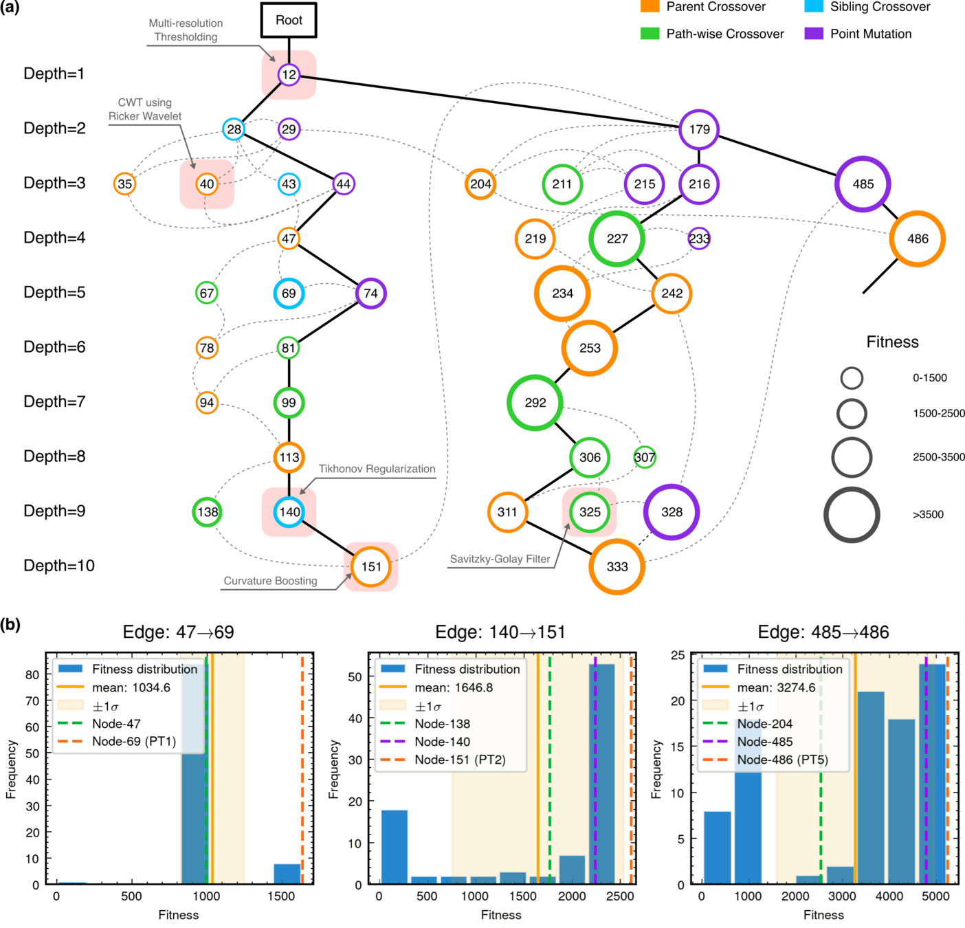
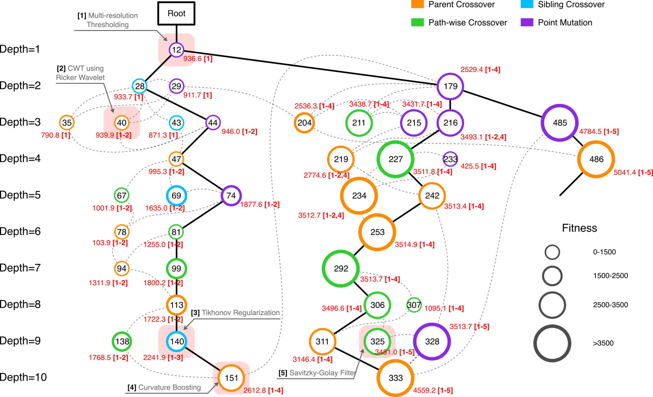
MCTS Algorithmic Evolution Pathway
MCTS Algorithmic Evolution Pathway
hewang@ucas.ac.cn
hewang@ucas.ac.cn
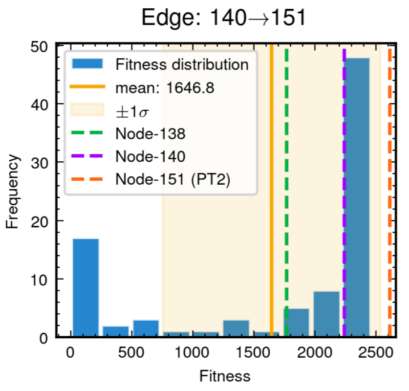
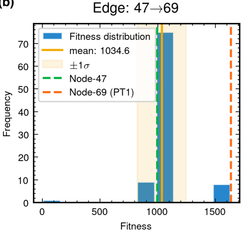
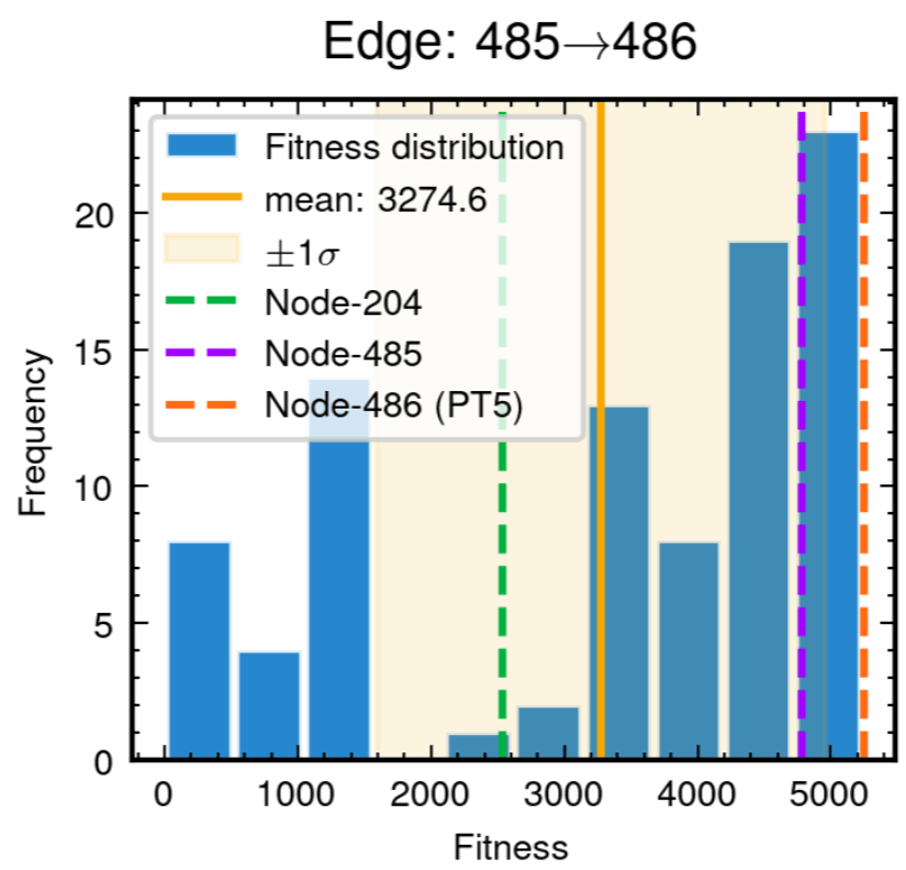
Edge robustness analysis for three critical evolutionary transitions.
52.8% achieving superior fitness with 100% Tikhonov regularization inheritance
89.3% variants exceeding preceding node performance
70.7% variants outperforming node 204, 25.0% surpassing node 485
Integrated Architecture Validation
Contributions of knowledge synthesis
hewang@ucas.ac.cn
LLM Model Selection and Robustness Analysis
o3-mini-medium
o1-2024-12-17
gpt-4o-2024-11-20
claude-3-7-sonnet-20250219-thinking
59.1%
AAD for GW detection Guided by LLM-informed Evo-MCTS
115%
Integrated Architecture Validation
Contributions of knowledge synthesis
hewang@ucas.ac.cn
59.1%
### External Knowledge Integration
1. **Non-linear** Processing Core Concepts:
    - Signal Transformation:
        * Non-linear vs linear decomposition
        * Adaptive threshold mechanisms
        * Multi-scale analysis

    - Feature Extraction:
        * Phase space reconstruction
        * Topological data analysis
        * Wavelet-based detection

    - Statistical Analysis:
        * Robust estimators
        * Non-Gaussian processes
        * Higher-order statistics

2. Implementation Principles:
    - Prioritize adaptive over fixed parameters
    - Consider local vs global characteristics
- Balance computational cost with accuracy“东方”超算系统(ORISE,北京)
hewang@ucas.ac.cn
第三方大模型推理服务
Interpretable Gravitational Wave Data Analysis with DL and LLMs
hewang@ucas.ac.cn
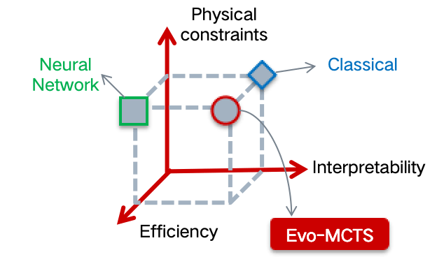
Our Mission: To create transparent AI systems that combine physics-based interpretability with deep learning capabilities
Interpretable AI Approach
The best of both worlds
Input
Physics-Informed
Algorithm
(High interpretability)
Output
Example: Evo-MCTS, AlphaEvolve
AI Model
Physics
Knowledge
Traditional Physics Approach
Input
Human-Designed Algorithm
(Based on human insight)
Output
Example: Matched Filtering, linear regression
Black-Box AI Approach
Input
AI Model
(Low interpretability)
Output
Examples: CNN, AlphaGo, DINGO
Data/
Experience
Data/
Experience
🎯 OUR WORK
What do we think about LLMs in scientific computing?
Interpretable Gravitational Wave Data Analysis with DL and LLMs
hewang@ucas.ac.cn
任何算法的设计问题都可被看作是一个优化问题
Interpretable Gravitational Wave Data Analysis with DL and LLMs
hewang@ucas.ac.cn
What are our thoughts on LLMs?
Product vs. Innovation
Interpretable Gravitational Wave Data Analysis with DL and LLMs
hewang@ucas.ac.cn
What are our thoughts on LLMs?
\(\Rightarrow\) Non-bias Objects? (Statistical Inference)
\(\Rightarrow\) GW / Cosmology Modeling (Discovering)
for _ in range(num_of_audiences):
    print('Thank you for your attention! 🙏')
\(\Rightarrow\) Domain-aware LLMs (Post-training)
\(\Rightarrow\) External knowledge powered (Test-time Scaling)
Preliminary
By He Wang
2025/12/09 14:00-15:00 “LlM and Science”Program @ITP-CAS


