


He Wang PRO
Knowledge increases by sharing but not by saving.
He Wang (王赫)
hewang@ucas.ac.cn
Beijing Normal University
International Centre for Theoretical Physics Asia-Pacific (ICTP-AP), UCAS
Taiji Laboratory for Gravitational Wave Universe (Beijing/Hangzhou), UCAS
On behave of KAGRA collaboration
The 12th KAGRA international workshop (KIW-12) | May 27, 2025 @SHAO
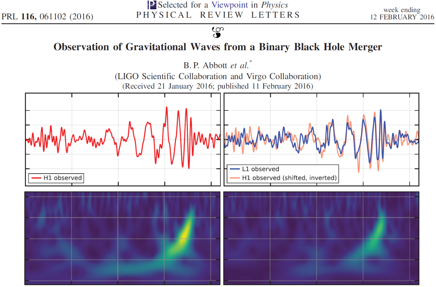
Gravitational waves (GW) are a strong field effect in General Relativity, ripples in the fabric of spacetime caused by accelerating massive objects.
GW Data Characteristics
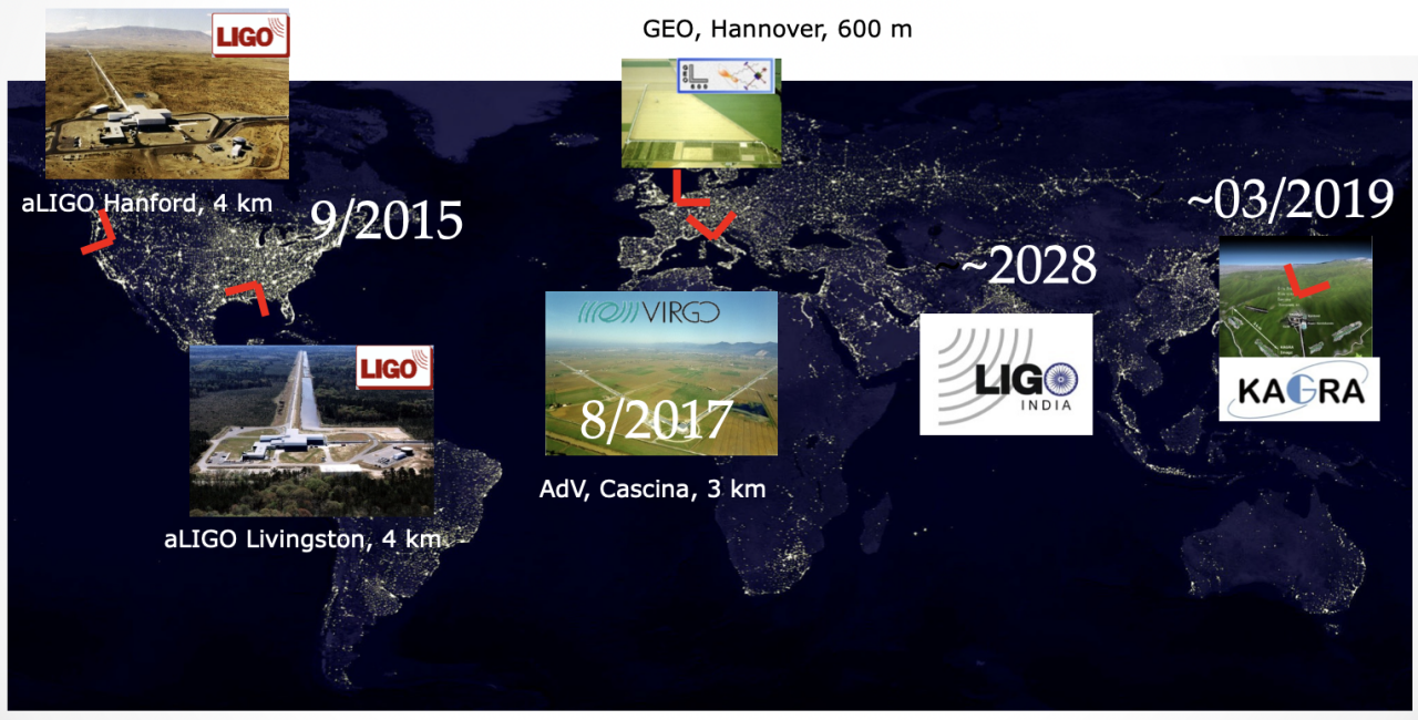
LIGO-VIRGO-KAGRA
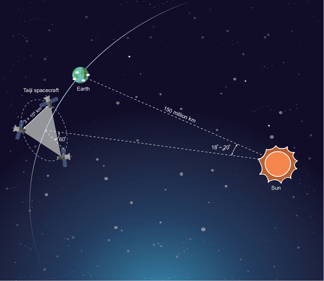
LISA Project
Noise: non-Gaussian and non-stationary
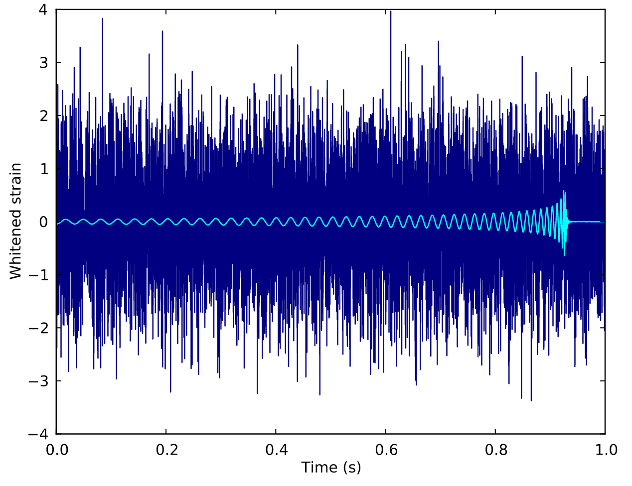
Signal challenges:
(Earth-based) A low signal-to-noise ratio (SNR) which is typically about 1/100 of the noise amplitude (-60 dB).
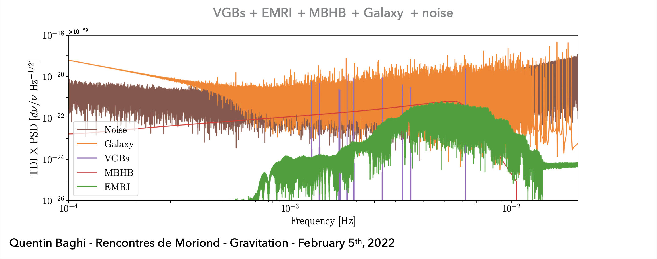
(Space-based) A superposition of all GW signals (e.g.: 104 of GBs, 10~102 of SMBHs, and 10~103 of EMRIs, etc.) received during the mission's observational run.
Matched Filtering Techniques (匹配滤波方法)
In Gaussian and stationary noise environments, the optimal linear algorithm for extracting weak signals
Statistical Approaches
Frequentist Testing:
Bayesian Testing:
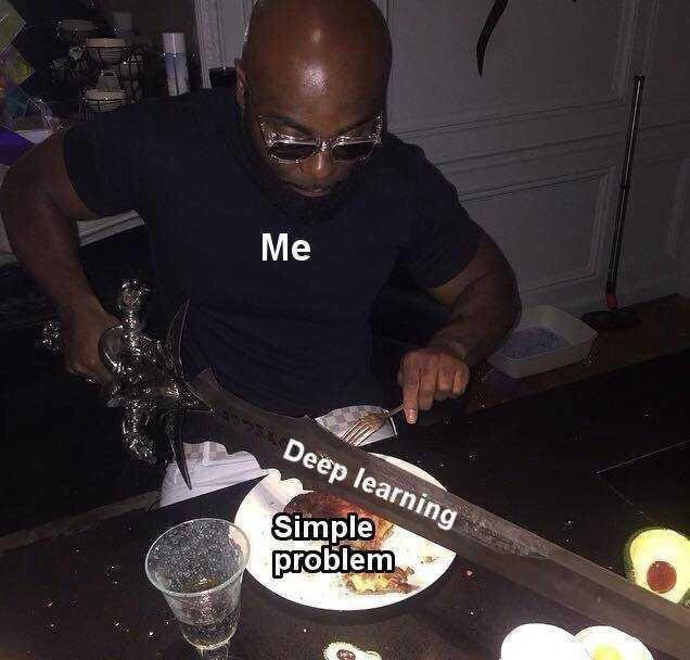
Interpretable Gravitational Wave Data Analysis with DL and LLMs
Interpretable Gravitational Wave Data Analysis with DL and LLMs
Let's be honest about our motivations... 😉
The perfectly valid "scientific" reasons:
Credit: Chris Messenger (MLA meeting,, Jan 2025)
Interpretable Gravitational Wave Data Analysis with DL and LLMs
The core motivations behind nearly all AI+GW research
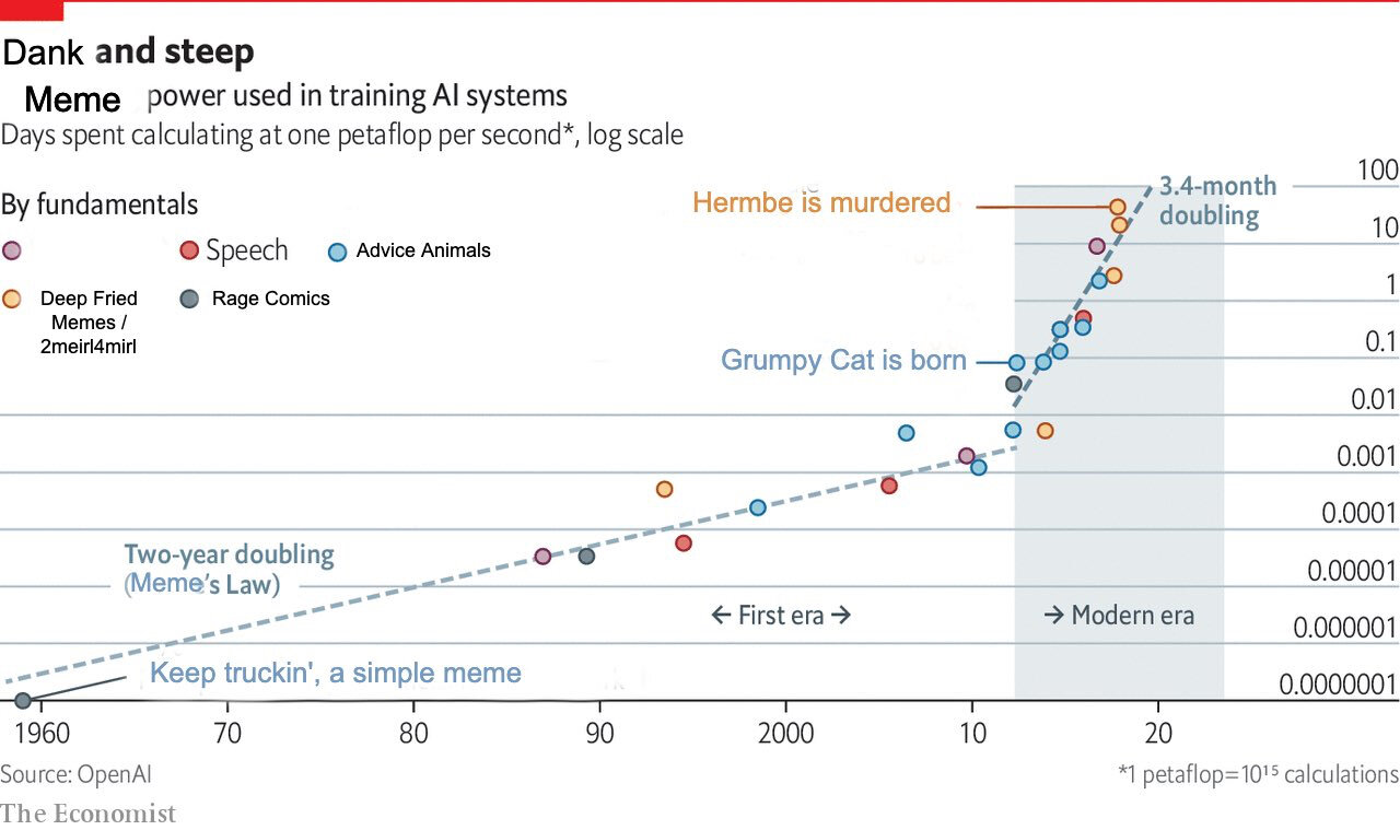
So much data, so little time!
• Bayesian parameter estimation
• Replaces computationally intensive components
Consistently outperforms traditional approaches
• Unmodelled burst searches
• Continuous GW searches
Provides deeper insights into complex problems
• Reveals patterns through interpretability
• Enables previously impractical approaches
* When properly trained and validated on appropriate datasets
Credit: Chris Messenger (MLA meeting,, Jan 2025)
Key question: If an ML (or any) analysis doesn't do 1 or more of these things, then from a scientific perspective,
what is the point?
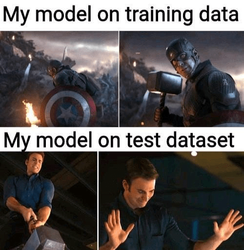
Interpretable Gravitational Wave Data Analysis with DL and LLMs
The reality of ML in scientific research is more nuanced
No: We need to think more critically
Twitter: @DeepLearningAI_
Interpretable Gravitational Wave Data Analysis with DL and LLMs
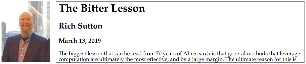
The mathematical inevitability and the path to understanding
The existence theorem that guarantees solutions
The solution is mathematically guaranteed — our challenge is finding the path to it
Machine learning will win in the long run
AI models still have vast potential compared to the human brain's efficiency. Beating traditional methods is mathematically inevitable given sufficient resources.
The question is not if AI/ML will win, but how
Understanding AI's inner workings is the real challenge, not proving its capabilities.
That's where we can learn something exciting with Foundation Models.
Interpretable Gravitational Wave Data Analysis with DL and LLMs
Bias:参考Sage
可解释性:feature extraction, Interpolation
LLM:
Detection
Inference
AHD
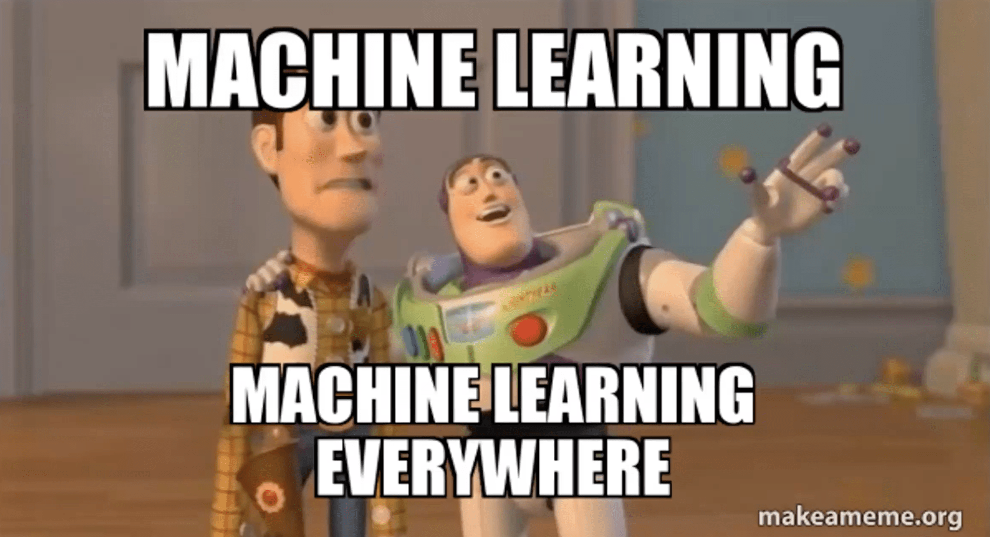
AI is taking over the world... literally everywhere
Interpretable Gravitational Wave Data Analysis with DL and LLMs
The core motivations behind nearly all AI+GW research
So much data, so little time!
• Bayesian parameter estimation
• Replaces computationally intensive components
Consistently outperforms traditional approaches
• Unmodelled burst searches
• Continuous GW searches
Provides deeper insights into complex problems
• Reveals patterns through interpretability
• Enables previously impractical approaches
* When properly trained and validated on appropriate datasets
Credit: Chris Messenger (MLA meeting,, Jan 2025)
Interpretable Gravitational Wave Data Analysis with DL and LLMs
Uncovering the "black box" to reveal
how AI actually processes GW strain data
Interpretable Gravitational Wave Data Analysis with DL and LLMs
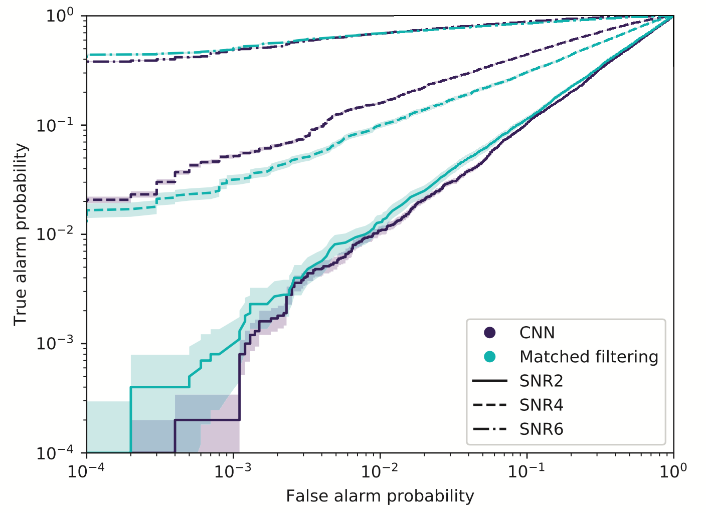
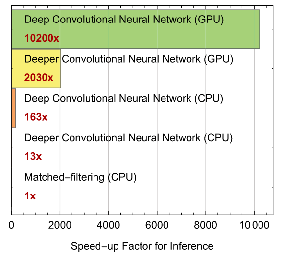
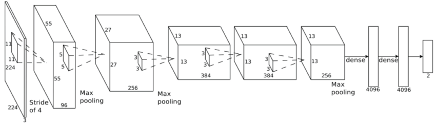
Core Insight from Computer Vision
Performance Analysis
Pioneering Research Publications
PRL, 2018, 120(14): 141103.
PRD, 2018, 97(4): 044039.
Interpretable Gravitational Wave Data Analysis with DL and LLMs
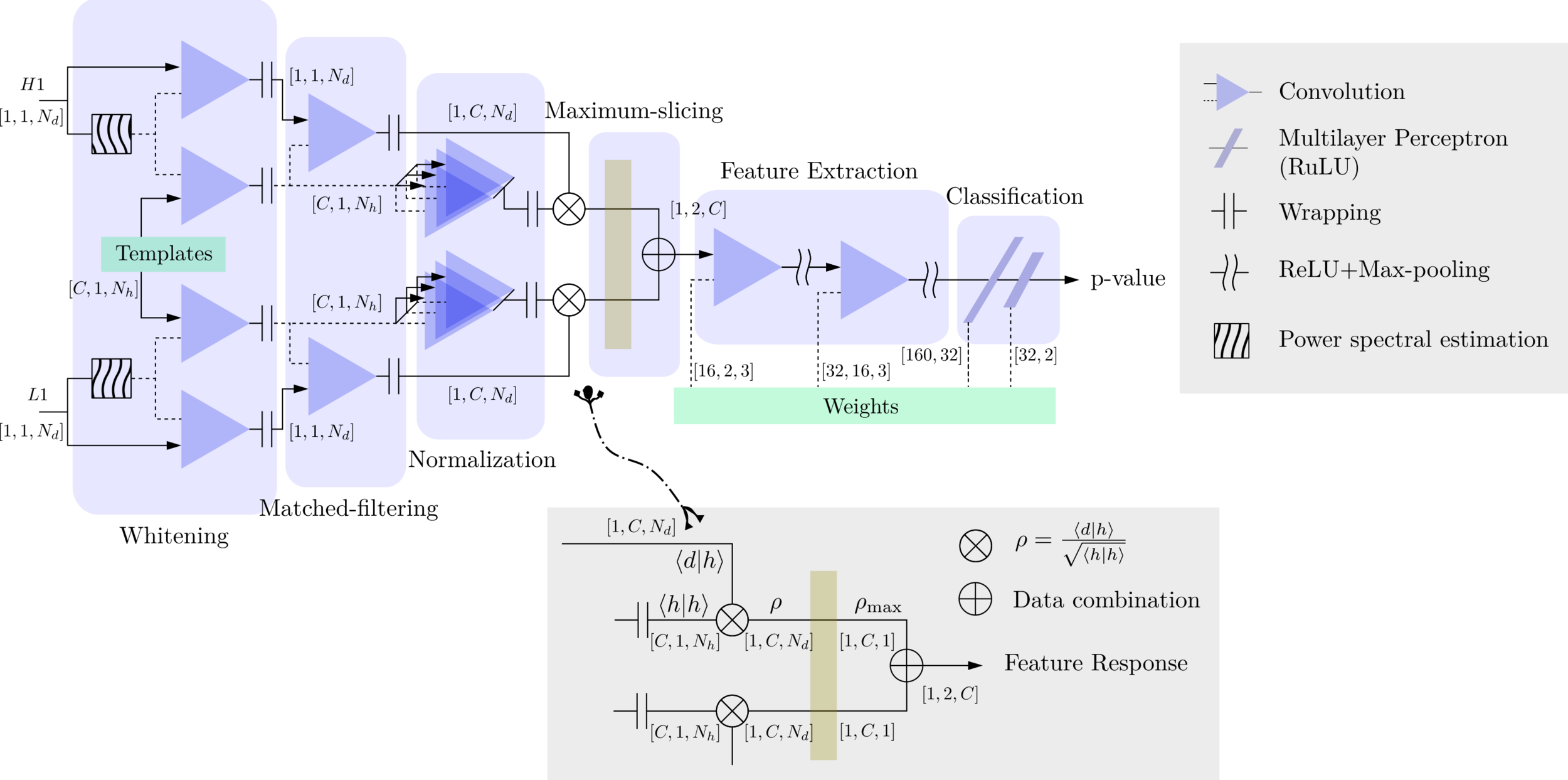
Matched-filtering Convolutional Neural Network (MFCNN)
HW, SC Wu, ZJ CAO, et al. PRD 101, 10 (2020): 104003
Convolutional Neural Network (ConvNet or CNN)
feature extraction
classifier
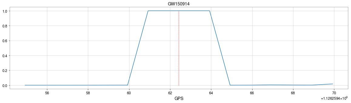
>> Is it matched-filtering ?
>> Wait, It can be matched-filtering!
GW150914
GW150914
Interpretable Gravitational Wave Data Analysis with DL and LLMs
Universal Approximation Theorem: Existence Theorem
Beyond Speed: Generalization and Explainability
Convolutional Neural Network (ConvNet or CNN)
Matched-filtering Convolutional Neural Network (MFCNN)
He Wang, et al. PRD 101, 10 (2020): 104003
GW150914
GW150914
Interpretable Gravitational Wave Data Analysis with DL and LLMs
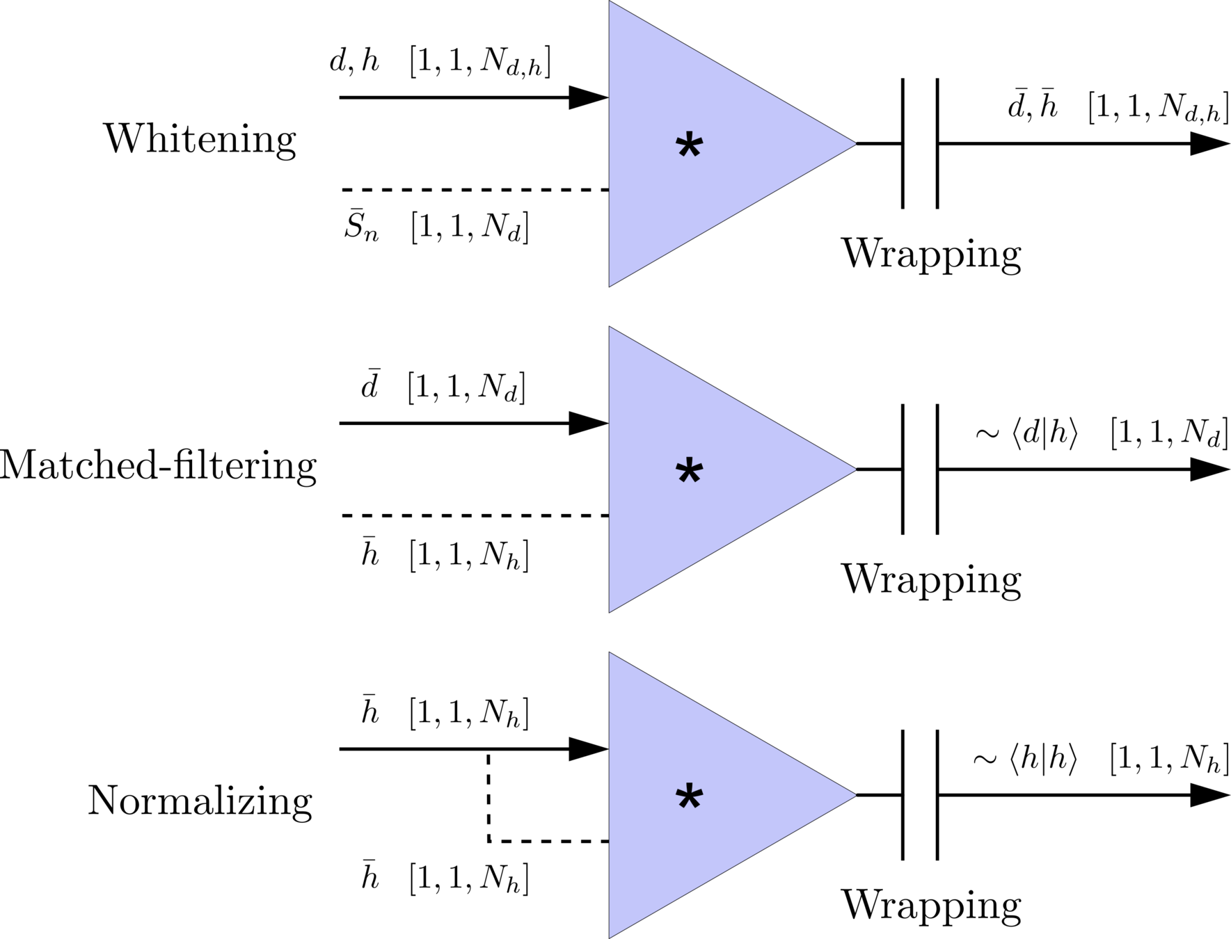
Transform matched-filtering method from frequency domain to time domain.
The square of matched-filtering SNR for a given data \(d(t) = n(t)+h(t)\):
\(S_n(|f|)\) is the one-sided average PSD of \(d(t)\)
where
Deep Learning Framework
Time Domain
(matched-filtering)
(normalizing)
(whitening)
Frequency Domain
Interpretable Gravitational Wave Data Analysis with DL and LLMs
Transform matched-filtering method from frequency domain to time domain.
The square of matched-filtering SNR for a given data \(d(t) = n(t)+h(t)\):
\(S_n(|f|)\) is the one-sided average PSD of \(d(t)\)
where
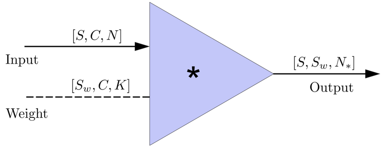
Deep Learning Framework
FYI: \(N_\ast = \lfloor(N-K+2P)/S\rfloor+1\)
(A schematic illustration for a unit of convolution layer)
Time Domain
(matched-filtering)
(normalizing)
(whitening)
Frequency Domain
Interpretable Gravitational Wave Data Analysis with DL and LLMs
import mxnet as mx
from mxnet import nd, gluon
from loguru import logger

def MFCNN(fs, T, C, ctx, template_block, margin, learning_rate=0.003):
    logger.success('Loading MFCNN network!')
    net = gluon.nn.Sequential()
    with net.name_scope():
        net.add(MatchedFilteringLayer(mod=fs*T, fs=fs,
                                      template_H1=template_block[:,:1],
                                      template_L1=template_block[:,-1:]))
        net.add(CutHybridLayer(margin = margin))
        net.add(Conv2D(channels=16, kernel_size=(1, 3), activation='relu'))
        net.add(MaxPool2D(pool_size=(1, 4), strides=2))
        net.add(Conv2D(channels=32, kernel_size=(1, 3), activation='relu'))
        net.add(MaxPool2D(pool_size=(1, 4), strides=2))
        net.add(Flatten())
        net.add(Dense(32))
        net.add(Activation('relu'))
        net.add(Dense(2))
	# Initialize parameters of all layers
    net.initialize(mx.init.Xavier(magnitude=2.24), ctx=ctx, force_reinit=True)
    return net
1 sec duration
35 templates used
Explainable AI Approach
Matched-filtering Convolutional Neural Network (MFCNN)
The available codes (2019): https://gist.github.com/iphysresearch/a00009c1eede565090dbd29b18ae982c
HW, SC Wu, ZJ CAO, et al. PRD 101, 10 (2020): 104003
Interpretable Gravitational Wave Data Analysis with DL and LLMs
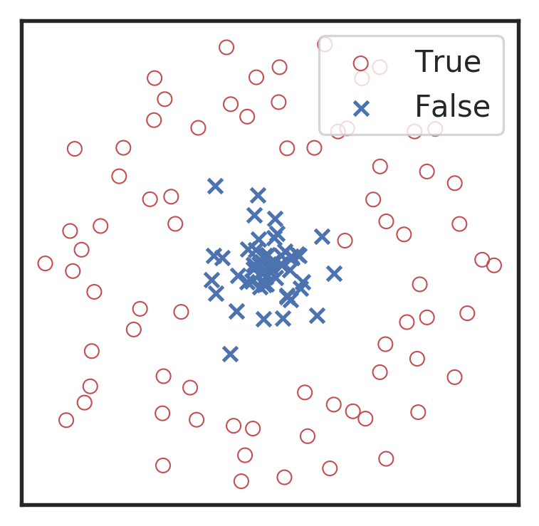
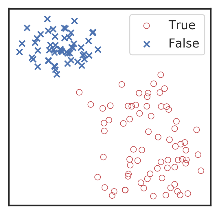
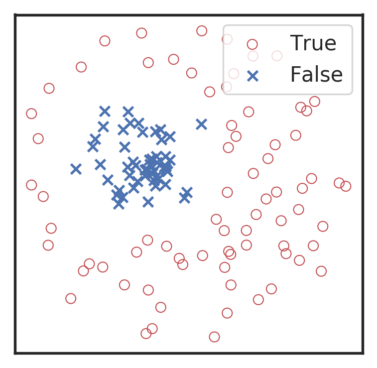
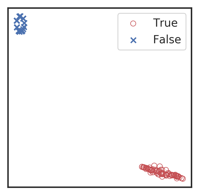
Visualization for the high-dimensional feature maps of learned network in layers for bi-class using t-SNE.
feature extraction
Convolutional Neural Network (ConvNet or CNN)
classifier
Is there GW or non-GW in it?
GW + noise / noise
Chapter 4, PhD thesis (2020):
https://iphysresearch.github.io/PhDthesis_html/C4/#45
Interpretable Gravitational Wave Data Analysis with DL and LLMs
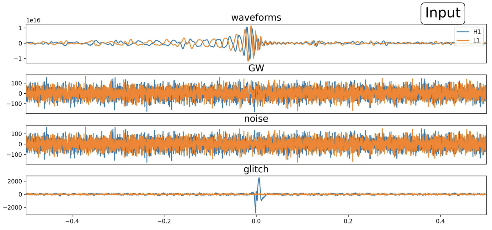
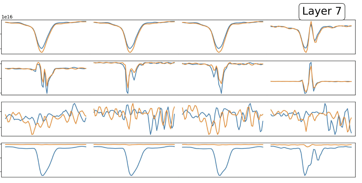
signal
noise
signal + noise
glitch_H1 + noise
Jun Tian, HW, et al. In Preparation (2025)
Is there GW or non-GW in it?
feature extraction
Convolutional Neural Network (ConvNet or CNN)
classifier
Interpretable Gravitational Wave Data Analysis with DL and LLMs
signal
noise
signal + noise
glitch_H1 + noise
Jun Tian, HW, et al. In Preparation (2025)
Is there GW or non-GW in it?
feature extraction
Convolutional Neural Network (ConvNet or CNN)
classifier
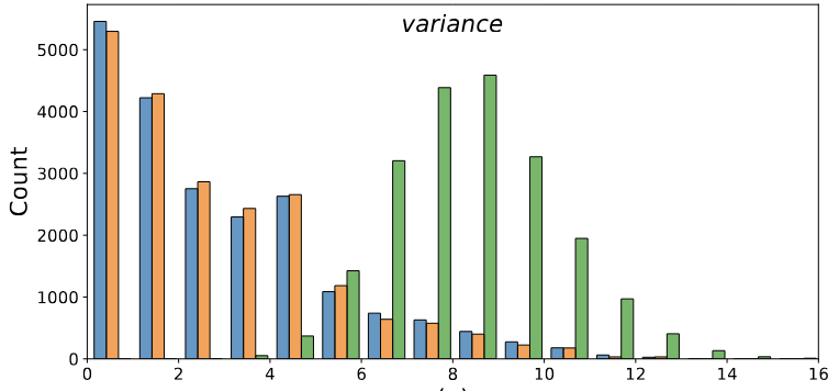
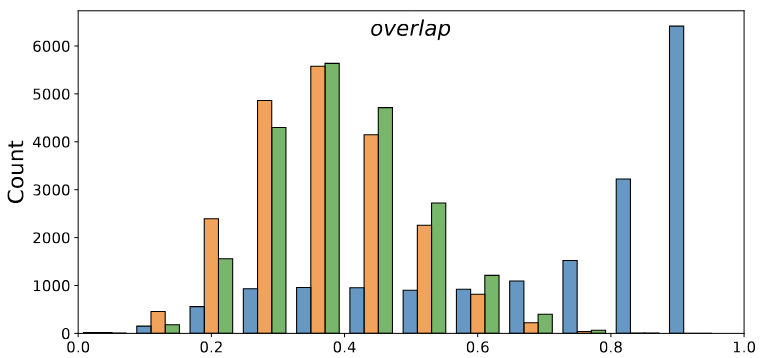
Key insight: At test time, one can easily construct statistics to differentiate between signal, noise, and glitches
Interpretable Gravitational Wave Data Analysis with DL and LLMs
Jun Tian, HW, et al. In Preparation (2025)
Proformance: Is there GW or non-GW in the data?
GW / noise + Glitch
GW / noise / Glitch
GW / noise
GW / noise / Glitch
GW / noise
Random
Forest
Interpretable Gravitational Wave Data Analysis with DL and LLMs
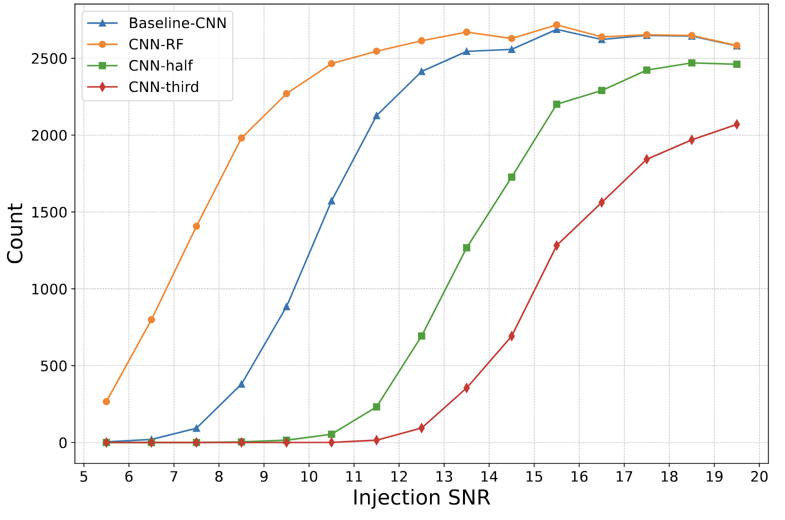
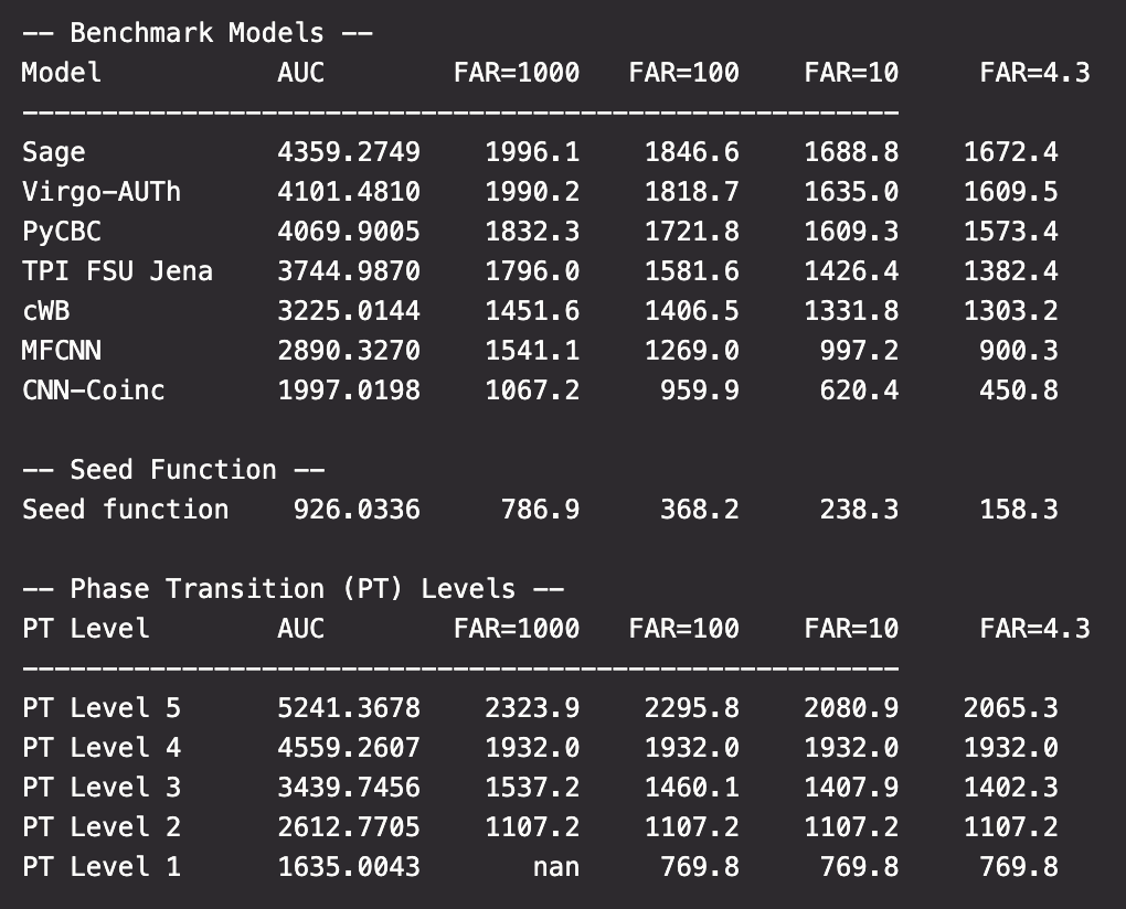
Benchmark Results
Publications
Key Findings
Note on Benchmark Limitations:
Outperforming PyCBC doesn't conclusively prove that matched filtering is inferior to AI methods. This is both because the dataset represents a specific distribution and because PyCBC settings could be further optimized for this particular benchmark.
arXiv:2501.13846 [gr-qc]
Phys. Rev. D 107, 023021 (2023)
Interpretable Gravitational Wave Data Analysis with DL and LLMs
AI Model Denoising
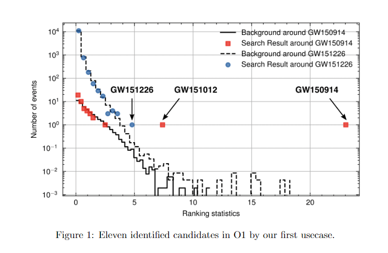
Our Model's Detection Statistics
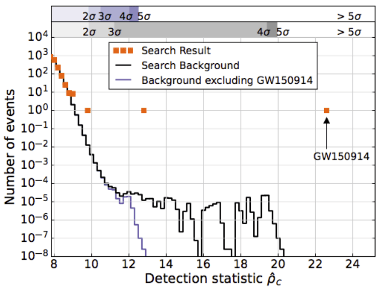
LVK Official Detection Statistics
Signal denoising visualization using our deep learning model (Transformer-based)
Detection statistics from our AI model showing O1 events
HW et al 2024 MLST 5 015046
GW151226
GW151012
Official detection statistics from LVK collaboration
LVK. PRD (2016). arXiv:1602.03839
Interpretable Gravitational Wave Data Analysis with DL and LLMs
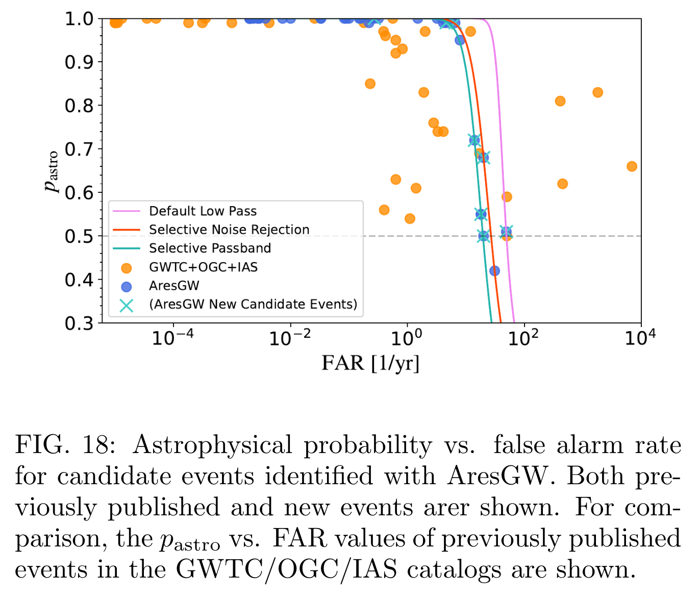
arXiv:2407.07820 [gr-qc]
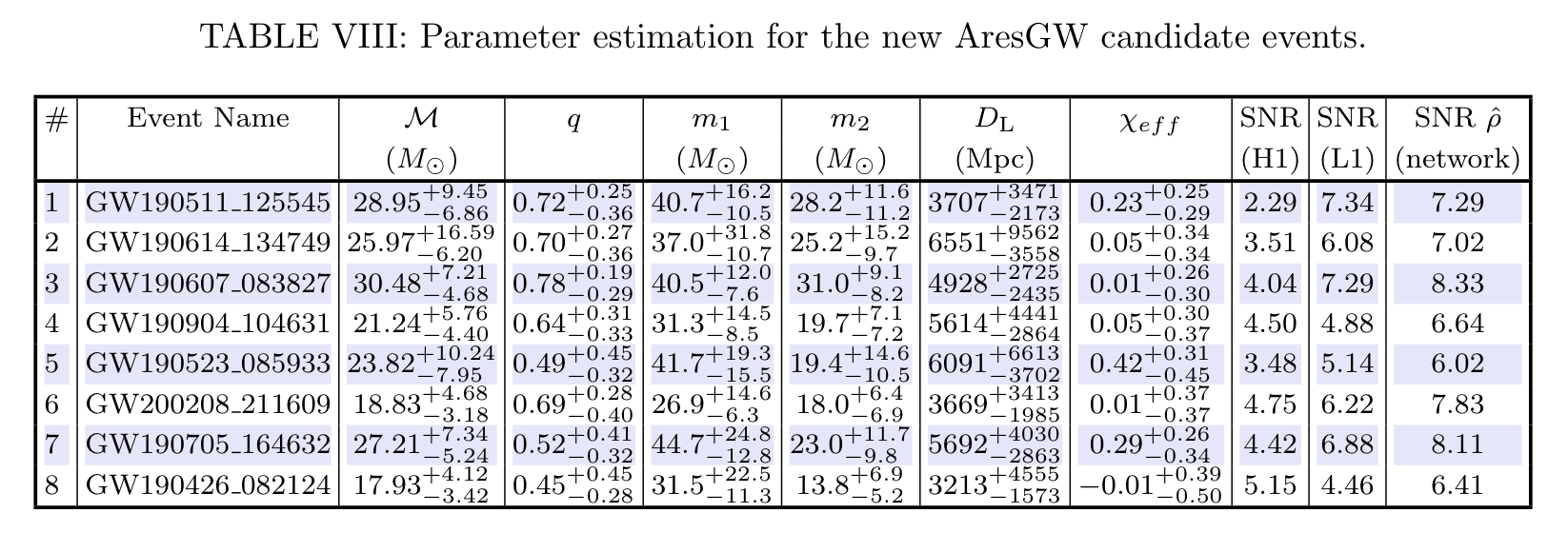
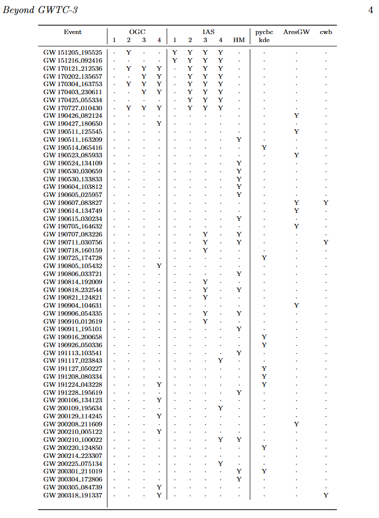
Recent AI Discoveries & Validation Hurdles:
Search
PE
Rate
Key Insight:
Interpretable Gravitational Wave Data Analysis with DL and LLMs
Recent AI Discoveries & Validation Hurdles:
Search
PE
Rate
Key Insight:
Credit: DCC-XXXXXXXX
Interpretable Gravitational Wave Data Analysis with DL and LLMs
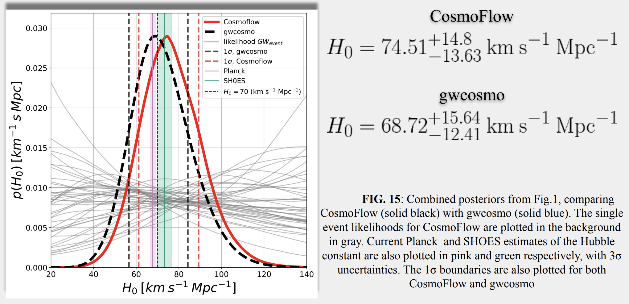
Parameter Estimation Challenges with AI Models:
arXiv:2404.14286
Phys. Rev. D 109, 123547 (2024)
Interpretable Gravitational Wave Data Analysis with DL and LLMs
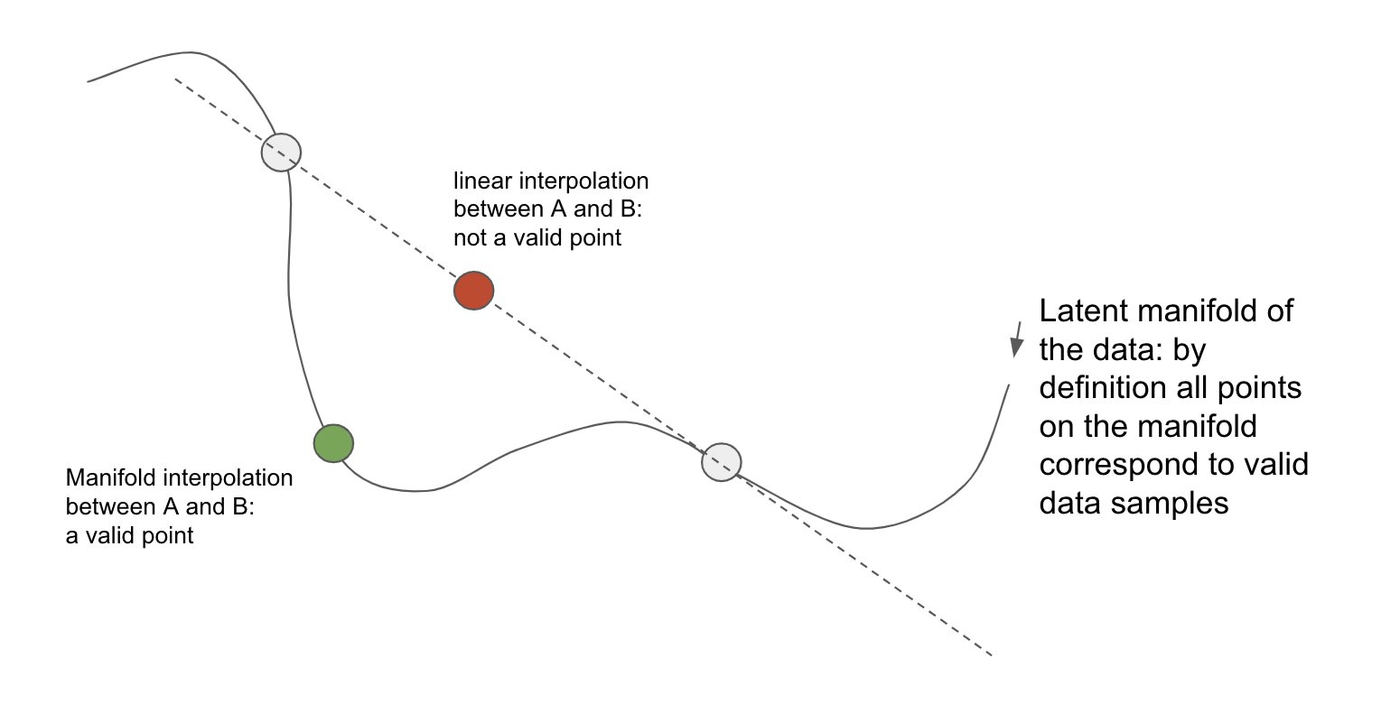
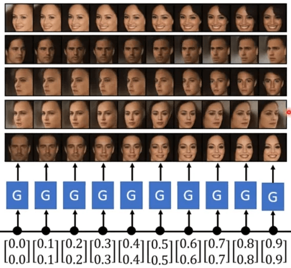
Representation Space Interpolation
Core Insights: Generative models' ability to perform accurate statistical inference can be understood as manifold learning rather than mere density estimation:
Generative models don't memorize examples, but learn a continuous manifold
where similar concepts lie near each other. Statistical inference becomes
a form of navigation through this learned representation space.
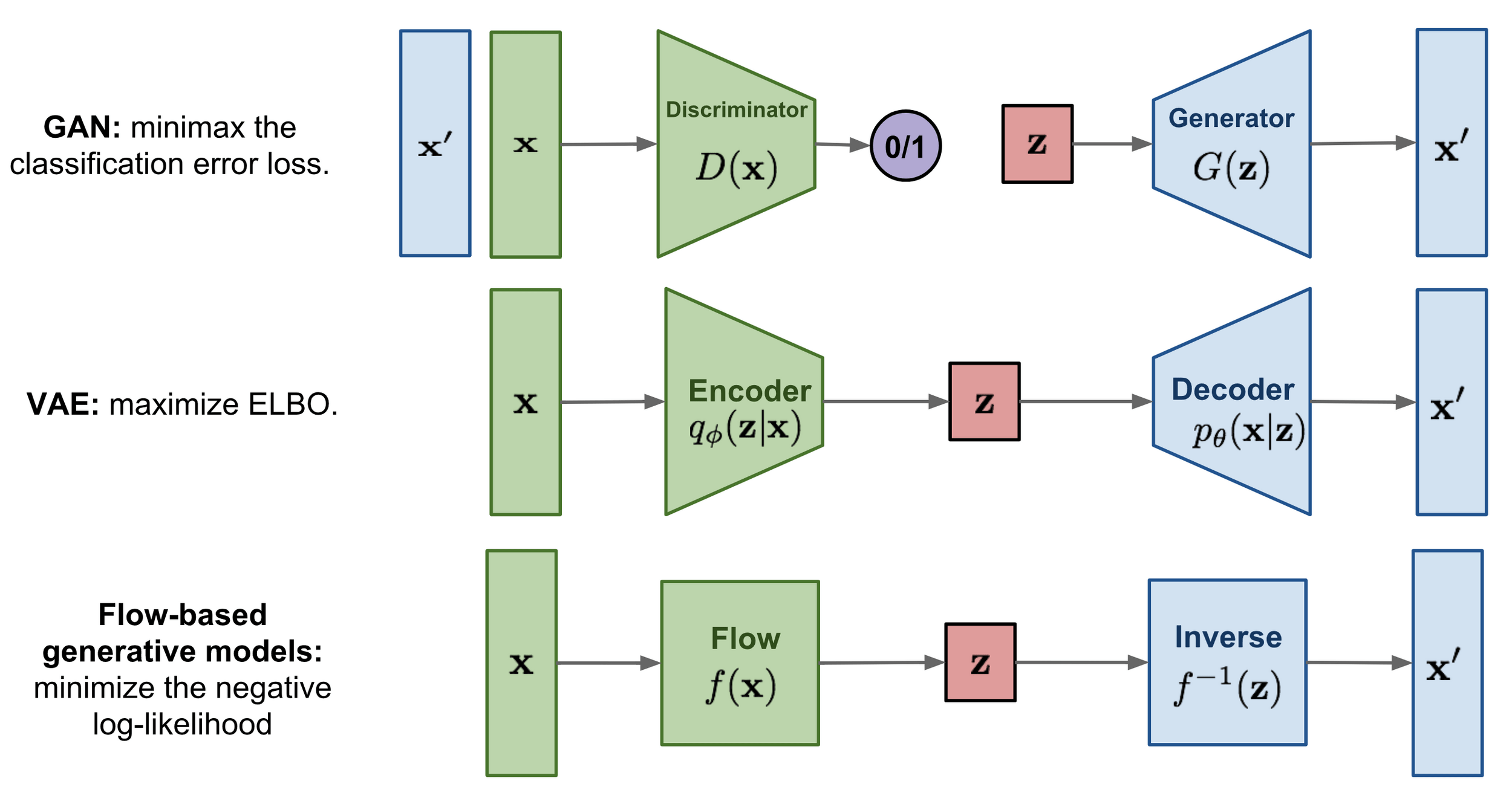
CVAE
Encodes data into latent space, enabling conditional generation
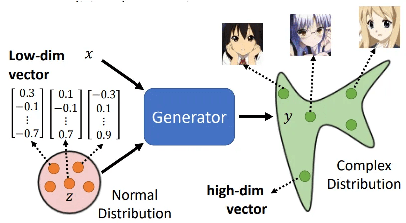
Flow-based
Transforms simple distributions into complex ones via invertible mappings
Interpretable Gravitational Wave Data Analysis with DL and LLMs
The core driving force of AI4Sci largely lies in its “interpolation” generalization capabilities, showcasing its powerful complex modeling abilities.
From 李宏毅
Interpretable Gravitational Wave Data Analysis with DL and LLMs
The core driving force of AI4Sci largely lies in its “interpolation” generalization capabilities, showcasing its powerful complex modeling abilities.
Interpretable Gravitational Wave Data Analysis with DL and LLMs
Test of General Relatively
2403.18936
Key Trust Factors:
Traditional Physics Approach
Input
Human-Designed Algorithm
(Based on human insight)
Output
Example: Matched Filtering,
Linear Regression
Black-Box AI Approach
Input
AI Model
(Low interpretability)
Output
Examples: CNN, AlphaGo, DINGO
Key Challenge: How can we maintain the interpretability advantages of traditional models while leveraging the power of AI approaches?
Data/
Experience
Data/
Experience
Interpretable Gravitational Wave Data Analysis with DL and LLMs
Combining the interpretability of physics with the power of AI
Our Mission: To create transparent AI systems that combine physics-based interpretability with deep learning capabilities
Interpretable AI Approach
The best of both worlds
Input
Physics-Informed
Algorithm
(High interpretability)
Output
Example: Our Approach
(In Preparation)
AI Model
Physics
Knowledge
Traditional Physics Approach
Input
Human-Designed Algorithm
(Based on human insight)
Output
Example: Matched Filtering, linear regression
Black-Box AI Approach
Input
AI Model
(Low interpretability)
Output
Examples: CNN, AlphaGo, DINGO
Data/
Experience
Data/
Experience
Interpretable Gravitational Wave Data Analysis with DL and LLMs
Understanding the fundamental principles rather than seeking shortcuts
The true value of AI in gravitational wave science emerges not from quick implementation, but from patient cultivation of deep understanding. This journey requires time, thoughtfulness, and respect for fundamental principles.
The Path to Deeper Understanding
True algorithmic mastery requires patience and depth:
for _ in range(num_of_audiences):
    print('Thank you for your attention! 🙏')
hewang@ucas.ac.cn
Given the interpretability challenges we've explored,
how might we advance GW detection and parameter estimation while maintaining scientific rigor?
Given the interpretability challenges we've explored, how might we advance GW detection and parameter estimation while maintaining scientific rigor?
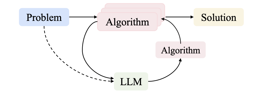
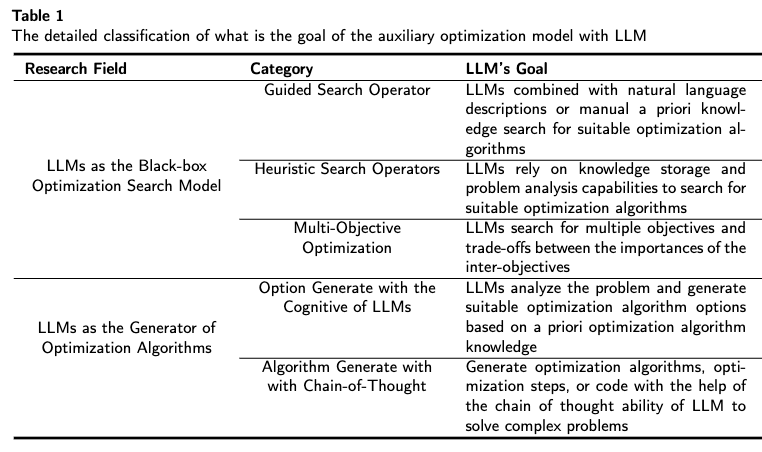
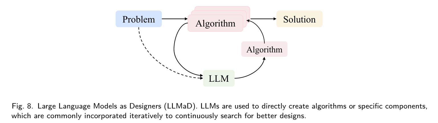
Automatic and Evolutionary Algorithm Heuristics for GW Detection using LLMs
A promising new approach combining the power of large language models with evolutionary algorithms to create interpretable, adaptive detection systems
For any complex task \(P\) (especially NP-hard problems), Automated Heuristic Design (AHD) searches for the optimal heuristic \(h^*\) within a heuristic space \(H\):
\(h^*=\underset{h \in H}{\arg \max } g(h) \)
The heuristic space \(H\) contains all feasible algorithmic solutions for task \(P\). Each heuristic \(h \in H\) maps from the set of task inputs \(I_P\) to corresponding solutions \(S_P\):
\(h: I_P \rightarrow S_P\)
Performance measure \(g(\cdot)\) evaluates each heuristic's effectiveness, \(g: H \rightarrow \mathbb{R}\). For minimization problems with objective function \(f: S_P \rightarrow \mathbb{R}\), we estimate performance by evaluating the heuristic instances \({ins}\in D \subseteq I_P\) on dataset \(D\) as follows:
\(g(h)=\mathbb{E}_{\boldsymbol{ins} \in D}[-f(h(\boldsymbol{ins}))]\)
arXiv.2410.14716
external_knowledge
(constraint)
Interpretable Gravitational Wave Data Analysis with DL and LLMs
HW et al., In preparation
import numpy as np
import scipy.signal as signal
def pipeline_v1(strain_h1: np.ndarray, strain_l1: np.ndarray, times: np.ndarray) -> tuple[np.ndarray, np.ndarray, np.ndarray]:
    def data_conditioning(strain_h1: np.ndarray, strain_l1: np.ndarray, times: np.ndarray) -> tuple[np.ndarray, np.ndarray, np.ndarray]:
        window_length = 4096
        dt = times[1] - times[0]
        fs = 1.0 / dt

        def whiten_strain(strain):
            strain_zeromean = strain - np.mean(strain)
            freqs, psd = signal.welch(strain_zeromean, fs=fs, nperseg=window_length,
                                       window='hann', noverlap=window_length//2)
            smoothed_psd = np.convolve(psd, np.ones(32) / 32, mode='same')
            smoothed_psd = np.maximum(smoothed_psd, np.finfo(float).tiny)
            white_fft = np.fft.rfft(strain_zeromean) / np.sqrt(np.interp(np.fft.rfftfreq(len(strain_zeromean), d=dt), freqs, smoothed_psd))
            return np.fft.irfft(white_fft)

        whitened_h1 = whiten_strain(strain_h1)
        whitened_l1 = whiten_strain(strain_l1)

        return whitened_h1, whitened_l1, times

    def compute_metric_series(h1_data: np.ndarray, l1_data: np.ndarray, time_series: np.ndarray) -> tuple[np.ndarray, np.ndarray]:
        fs = 1 / (time_series[1] - time_series[0])
        f_h1, t_h1, Sxx_h1 = signal.spectrogram(h1_data, fs=fs, nperseg=256, noverlap=128, mode='magnitude', detrend=False)
        f_l1, t_l1, Sxx_l1 = signal.spectrogram(l1_data, fs=fs, nperseg=256, noverlap=128, mode='magnitude', detrend=False)
        tf_metric = np.mean((Sxx_h1**2 + Sxx_l1**2) / 2, axis=0)
        gps_mid_time = time_series[0] + (time_series[-1] - time_series[0]) / 2
        metric_times = gps_mid_time + (t_h1 - t_h1[-1] / 2)

        return tf_metric, metric_times

    def calculate_statistics(tf_metric, t_h1):
        background_level = np.median(tf_metric)
        peaks, _ = signal.find_peaks(tf_metric, height=background_level * 1.0, distance=2, prominence=background_level * 0.3)
        peak_times = t_h1[peaks]
        peak_heights = tf_metric[peaks]
        peak_deltat = np.full(len(peak_times), 10.0)  # Fixed uncertainty value
        return peak_times, peak_heights, peak_deltat

    whitened_h1, whitened_l1, data_times = data_conditioning(strain_h1, strain_l1, times)
    tf_metric, metric_times = compute_metric_series(whitened_h1, whitened_l1, data_times)
    peak_times, peak_heights, peak_deltat = calculate_statistics(tf_metric, metric_times)

    return peak_times, peak_heights, peak_deltat
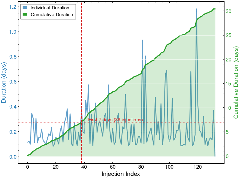
Input: H1 and L1 detector strains, time array | Output: Event times, significance values, and time uncertainties
external_knowledge
(constraint)
Problem: Pipeline Workflow
Optimization Target: Maximizing Area Under Curve (AUC) in the 1-1000Hz false alarms per-year range, balancing detection sensitivity and false alarm rates across algorithm generations
Interpretable Gravitational Wave Data Analysis with DL and LLMs
HW et al., In preparation
external_knowledge
(constraint)
Prompt Structure for Algorithm Evolution
This template guides the LLM to generate optimized gravitational wave detection algorithms by learning from comparative examples.
Key Components:
You are an expert in gravitational wave signal detection algorithms. Your task is to design heuristics that can effectively solve optimization problems.

{prompt_task}

I have analyzed two algorithms and provided a reflection on their differences.

[Worse code]
{worse_code}

[Better code]
{better_code}

[Reflection]
{reflection}

Based on this reflection, please write an improved algorithm according to the reflection.
First, describe the design idea and main steps of your algorithm in one sentence. The description must be inside a brace outside the code implementation. Next, implement it in Python as a function named '{func_name}'.
This function should accept {input_count} input(s): {joined_inputs}. The function should return {output_count} output(s): {joined_outputs}.
{inout_inf} {other_inf}

Do not give additional explanations.
One Prompt Template for MLGWSC1 Algorithm Synthesis
Interpretable Gravitational Wave Data Analysis with DL and LLMs
HW et al., In preparation
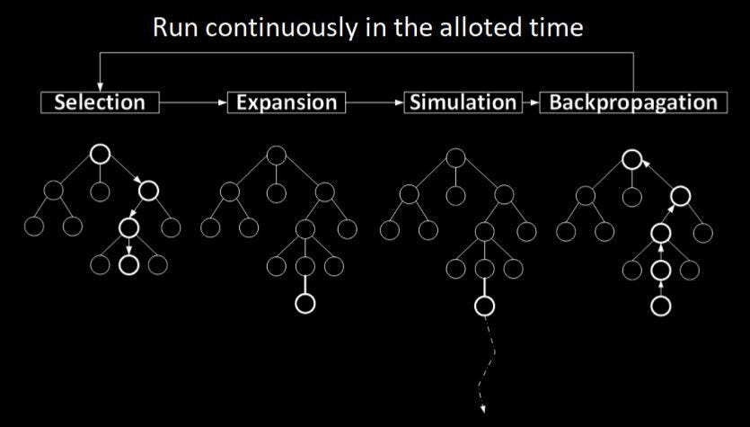
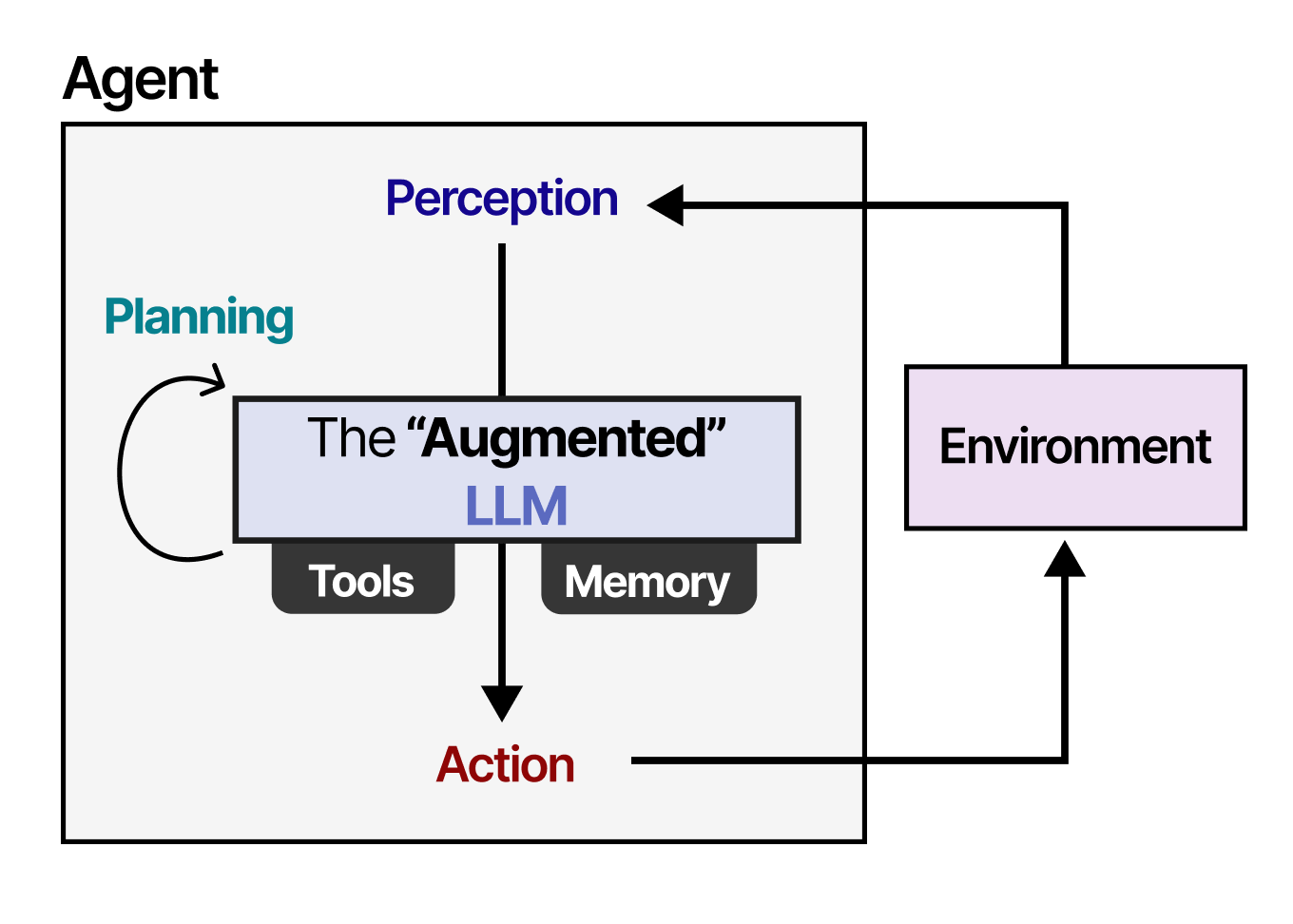
Monte Carlo Tree Search (MCTS)
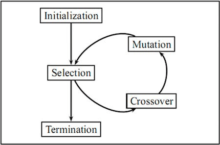
Evolutionary Algorithms
LLM Agents
Together, these approaches create a powerful framework for heuristic optimization of gravitational wave signal search algorithms
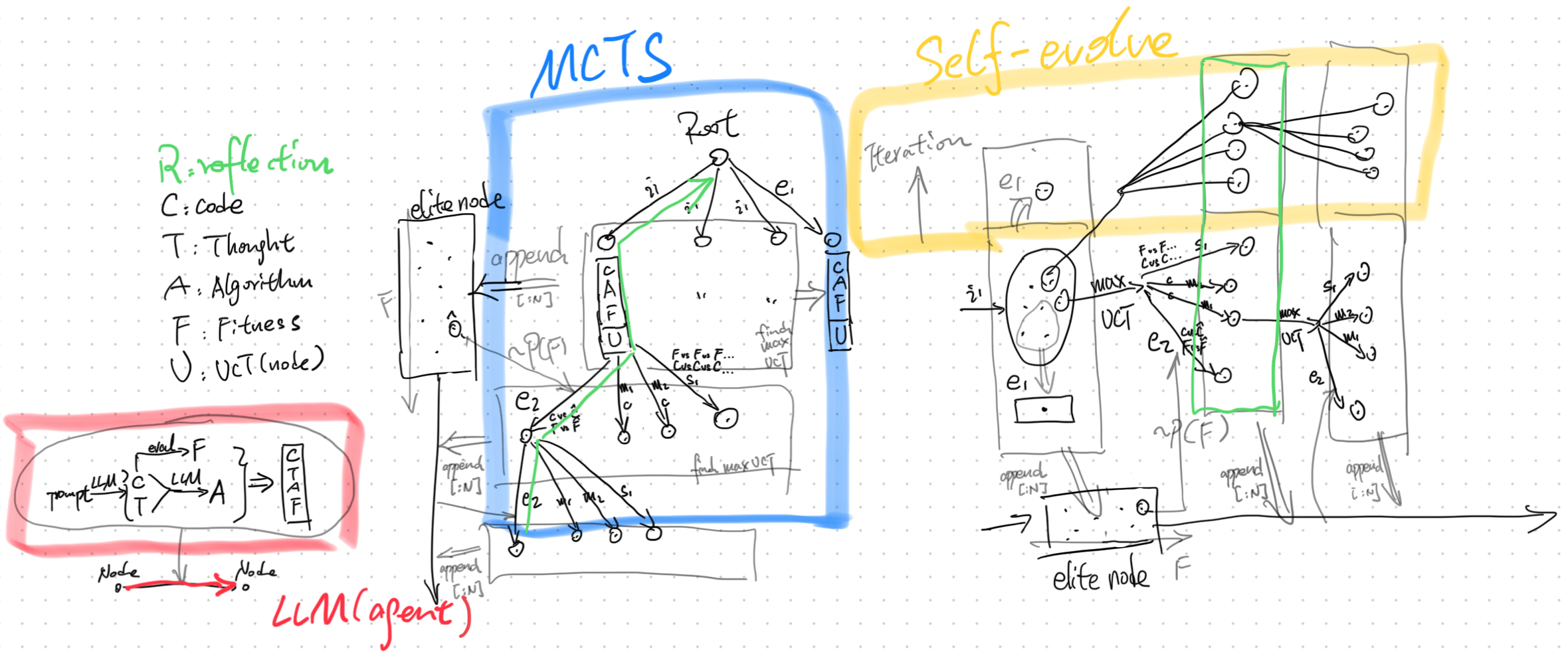
Interpretable Gravitational Wave Data Analysis with DL and LLMs
Proposed framework integrating MCTS decision-making, self-evolutionary optimization, and LLM agent guidance for gravitational wave signal search
With route/short/long-term reflection:《Thinking, Fast and Slow》
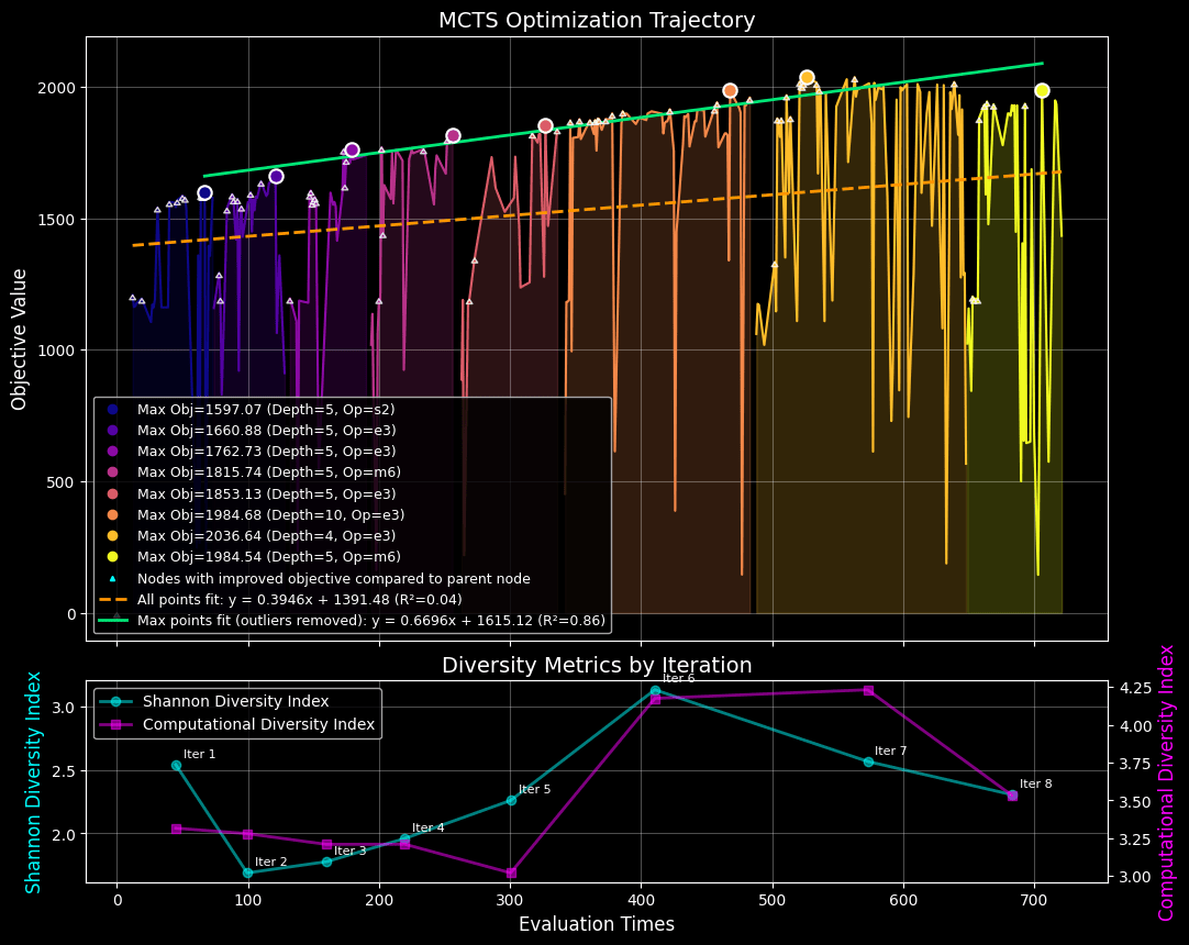
Preliminary Results (February 2025)
Interpretable Gravitational Wave Data Analysis with DL and LLMs
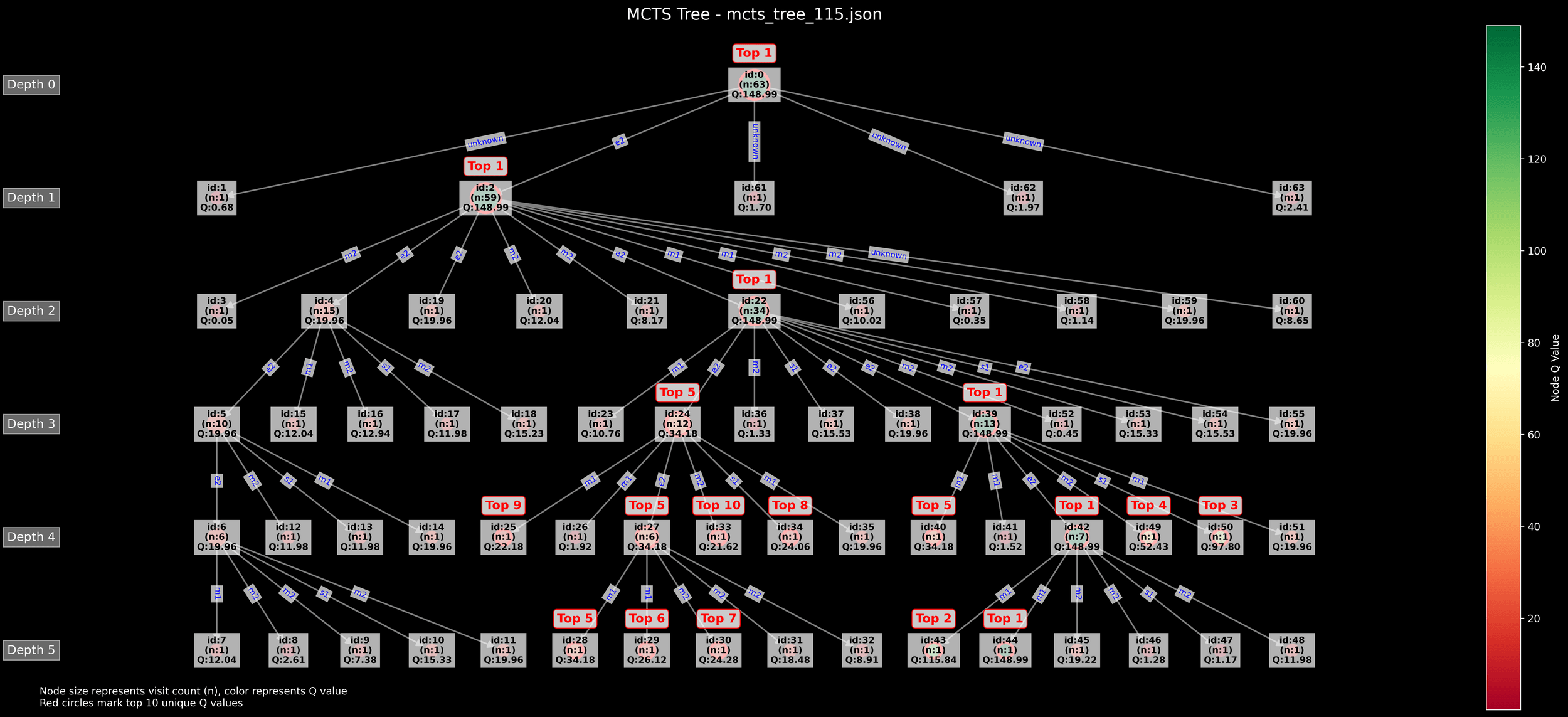
MLGWSC1 preliminary 结果
Tree-based representation of our framework's exploration path, where each node represents a unique algorithm variant generated during the optimization process
Node color intensity: Algorithm performance level | Connections: Algorithmic modifications | Tree depth: Iteration sequence
Interpretable Gravitational Wave Data Analysis with DL and LLMs
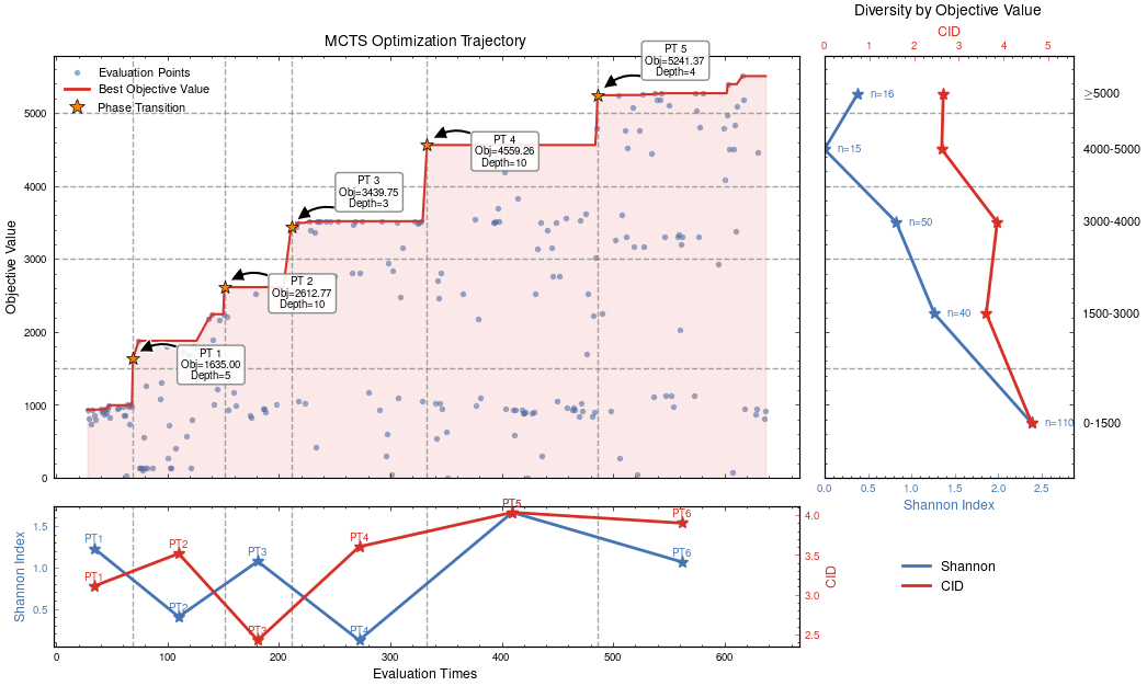
Preliminary Results (February 2025)
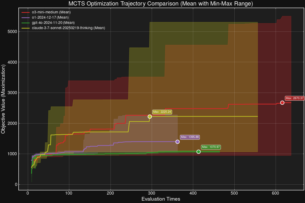
Optimization Progress & Algorithm Diversity
Interpretable Gravitational Wave Data Analysis with DL and LLMs
HW et al., In preparation
Pipeline Workflow
Diversity in Evolutionary Computation
Population encoding:
Pipeline Workflow
Interpretable Gravitational Wave Data Analysis with DL and LLMs
HW et al., In preparation
Refs of Benchmark Models
The algorithm first whitens and conditions dual-detector data by applying fixed-length (nperseg=256) Welch PSD estimation combined with a non-adaptive 0.5×tanh gain modulation, emphasizing spectral features where noise is minimal via an inverse dual‐detector weighting approach. It then computes a coherent time-frequency metric and extracts candidate gravitational wave events using cascaded multi-resolution thresholding and fixed-scale continuous wavelet transform (CWT) validation, propagating Gaussian uncertainty to refine each trigger’s timing accuracy.
The algorithm integrates adaptive median-based detrending and exponential adaptive whitening—where strain variance, spectral smoothing, and Tikhonov-regularized spectral inversion are prioritized—to produce a frequency-coherent metric that is further refined using both spectrogram phase coherence and local curvature boosting. It then employs a dynamically relaxed multi-resolution peak detection scheme, including dyadic CWT analysis and curvature checks, to robustly identify and validate candidate gravitational wave signals while balancing sensitivity against noise variability.
The algorithm begins by removing long-term nonstationarity via adaptive median filtering, then applies dynamic, frequency-dependent spectral whitening using an adaptive Kalman-inspired smoothing of the PSD to accentuate transients. It subsequently computes a coherent time-frequency metric through complex spectrogram cross-correlation and robust phase coherence, and finally identifies candidate gravitational wave signals via multi-resolution thresholding with CWT-based validation that emphasizes adaptive windowing and robust local uncertainty estimation.
This pipeline integrates robust median detrending and Kalman‐inspired PSD smoothing with gradient-adaptive whitening (via Savitzky–Golay filtering), emphasizing adaptive gain computations from high‐priority spectral PSD parameters while de-emphasizing global noise baseline variations. It then computes a coherent time-frequency metric—with axial second derivative curvature boosting and frequency‐conditioned regularization—and employs multi‐resolution thresholding using octave‐spaced dyadic wavelet validation to identify candidate gravitational wave events with precise timing uncertainty.
This pipeline robustly detrends and adaptively whitens the dual-channel gravitational wave data—with higher priority given to the adaptive PSD smoothing (via stationarity-based exponential smoothing and Savitzky–Golay spectral gradient scaling) and frequency-conditioned regularization—to compute a coherent time-frequency metric combining phase coherence and curvature boost. It then applies cascaded multi-resolution thresholding and octave-spaced Ricker wavelet validation with local uncertainty estimation to reliably isolate potential gravitational wave triggers, outputting their GPS time, significance, and timing uncertainty.
So, what went down during the Phase Transition (PT)?
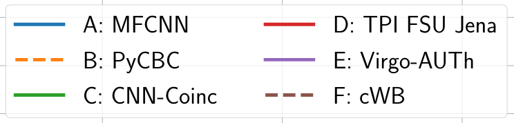
PyCBC (linear-core)
cWB (nonlinear-core)
Simple non-linear filters
CNN-like (highly non-linear)
Interpretable Gravitational Wave Data Analysis with DL and LLMs
HW et al., In preparation
import numpy as np
import scipy.signal as signal
from scipy.signal.windows import tukey
from scipy.signal import savgol_filter

def pipeline_v2(strain_h1: np.ndarray, strain_l1: np.ndarray, times: np.ndarray) -> tuple[np.ndarray, np.ndarray, np.ndarray]:
    """
    The pipeline function processes gravitational wave data from the H1 and L1 detectors to identify potential gravitational wave signals.
    It takes strain_h1 and strain_l1 numpy arrays containing detector data, and times array with corresponding time points.
    The function returns a tuple of three numpy arrays: peak_times containing GPS times of identified events,
    peak_heights with significance values of each peak, and peak_deltat showing time window uncertainty for each peak.
    """
    eps = np.finfo(float).tiny
    dt = times[1] - times[0]
    fs = 1.0 / dt
    # Base spectrogram parameters
    base_nperseg = 256
    base_noverlap = base_nperseg // 2
    medfilt_kernel = 101       # odd kernel size for robust detrending
    uncertainty_window = 5     # half-window for local timing uncertainty

    # -------------------- Stage 1: Robust Baseline Detrending --------------------
    # Remove long-term trends using a median filter for each channel.
    detrended_h1 = strain_h1 - signal.medfilt(strain_h1, kernel_size=medfilt_kernel)
    detrended_l1 = strain_l1 - signal.medfilt(strain_l1, kernel_size=medfilt_kernel)

    # -------------------- Stage 2: Adaptive Whitening with Enhanced PSD Smoothing --------------------
    def adaptive_whitening(strain: np.ndarray) -> np.ndarray:
        # Center the signal.
        centered = strain - np.mean(strain)
        n_samples = len(centered)
        # Adaptive window length: between 5 and 30 seconds
        win_length_sec = np.clip(n_samples / fs / 20, 5, 30)
        nperseg_adapt = int(win_length_sec * fs)
        nperseg_adapt = max(10, min(nperseg_adapt, n_samples))

        # Create a Tukey window with 75% overlap.
        tukey_alpha = 0.25
        win = tukey(nperseg_adapt, alpha=tukey_alpha)
        noverlap_adapt = int(nperseg_adapt * 0.75)
        if noverlap_adapt >= nperseg_adapt:
            noverlap_adapt = nperseg_adapt - 1

        # Estimate the power spectral density (PSD) using Welch's method.
        freqs, psd = signal.welch(centered, fs=fs, nperseg=nperseg_adapt,
                                  noverlap=noverlap_adapt, window=win, detrend='constant')
        psd = np.maximum(psd, eps)

        # Compute relative differences for PSD stationarity measure.
        diff_arr = np.abs(np.diff(psd)) / (psd[:-1] + eps)
        # Smooth the derivative with a moving average.
        if len(diff_arr) >= 3:
            smooth_diff = np.convolve(diff_arr, np.ones(3)/3, mode='same')
        else:
            smooth_diff = diff_arr

        # Exponential smoothing (Kalman-like) with adaptive alpha using PSD stationarity.
        smoothed_psd = np.copy(psd)
        for i in range(1, len(psd)):
            # Adaptive smoothing coefficient: base 0.8 modified by local stationarity (±0.05)
            local_alpha = np.clip(0.8 - 0.05 * smooth_diff[min(i-1, len(smooth_diff)-1)], 0.75, 0.85)
            smoothed_psd[i] = local_alpha * smoothed_psd[i-1] + (1 - local_alpha) * psd[i]

        # Compute Tikhonov regularization gain based on deviation from median PSD.
        noise_baseline = np.median(smoothed_psd)
        raw_gain = (smoothed_psd / (noise_baseline + eps)) - 1.0

        # Compute a causal-like gradient using the Savitzky-Golay filter.
        win_len = 11 if len(smoothed_psd) >= 11 else ((len(smoothed_psd)//2)*2+1)
        polyorder = 2 if win_len > 2 else 1
        delta_freq = np.mean(np.diff(freqs))
        grad_psd = savgol_filter(smoothed_psd, win_len, polyorder, deriv=1, delta=delta_freq, mode='interp')

        # Nonlinear scaling via sigmoid to enhance gradient differences.
        sigmoid = lambda x: 1.0 / (1.0 + np.exp(-x))
        scaling_factor = 1.0 + 2.0 * sigmoid(np.abs(grad_psd) / (np.median(smoothed_psd) + eps))

        # Compute adaptive gain factors with nonlinear scaling.
        gain = 1.0 - np.exp(-0.5 * scaling_factor * raw_gain)
        gain = np.clip(gain, -8.0, 8.0)

        # FFT-based whitening: interpolate gain and PSD onto FFT frequency bins.
        signal_fft = np.fft.rfft(centered)
        freq_bins = np.fft.rfftfreq(n_samples, d=dt)
        interp_gain = np.interp(freq_bins, freqs, gain, left=gain[0], right=gain[-1])
        interp_psd = np.interp(freq_bins, freqs, smoothed_psd, left=smoothed_psd[0], right=smoothed_psd[-1])
        denom = np.sqrt(interp_psd) * (np.abs(interp_gain) + eps)
        denom = np.maximum(denom, eps)
        white_fft = signal_fft / denom
        whitened = np.fft.irfft(white_fft, n=n_samples)
        return whitened

    # Whiten H1 and L1 channels using the adapted method.
    white_h1 = adaptive_whitening(detrended_h1)
    white_l1 = adaptive_whitening(detrended_l1)

    # -------------------- Stage 3: Coherent Time-Frequency Metric with Frequency-Conditioned Regularization --------------------
    def compute_coherent_metric(w1: np.ndarray, w2: np.ndarray) -> tuple[np.ndarray, np.ndarray]:
        # Compute complex spectrograms preserving phase information.
        f1, t_spec, Sxx1 = signal.spectrogram(w1, fs=fs, nperseg=base_nperseg,
                                              noverlap=base_noverlap, mode='complex', detrend=False)
        f2, t_spec2, Sxx2 = signal.spectrogram(w2, fs=fs, nperseg=base_nperseg,
                                               noverlap=base_noverlap, mode='complex', detrend=False)
        # Ensure common time axis length.
        common_len = min(len(t_spec), len(t_spec2))
        t_spec = t_spec[:common_len]
        Sxx1 = Sxx1[:, :common_len]
        Sxx2 = Sxx2[:, :common_len]

        # Compute phase differences and coherence between detectors.
        phase_diff = np.angle(Sxx1) - np.angle(Sxx2)
        phase_coherence = np.abs(np.cos(phase_diff))

        # Estimate median PSD per frequency bin from the spectrograms.
        psd1 = np.median(np.abs(Sxx1)**2, axis=1)
        psd2 = np.median(np.abs(Sxx2)**2, axis=1)

        # Frequency-conditioned regularization gain (reflection-guided).
        lambda_f = 0.5 * ((np.median(psd1) / (psd1 + eps)) + (np.median(psd2) / (psd2 + eps)))
        lambda_f = np.clip(lambda_f, 1e-4, 1e-2)
        # Regularization denominator integrating detector PSDs and lambda.
        reg_denom = (psd1[:, None] + psd2[:, None] + lambda_f[:, None] + eps)

        # Weighted phase coherence that balances phase alignment with noise levels.
        weighted_comp = phase_coherence / reg_denom

        # Compute axial (frequency) second derivatives as curvature estimates.
        d2_coh = np.gradient(np.gradient(phase_coherence, axis=0), axis=0)
        avg_curvature = np.mean(np.abs(d2_coh), axis=0)

        # Nonlinear activation boost using tanh for regions of high curvature.
        nonlinear_boost = np.tanh(5 * avg_curvature)
        linear_boost = 1.0 + 0.1 * avg_curvature

        # Cross-detector synergy: weight derived from global median consistency.
        novel_weight = np.mean((np.median(psd1) + np.median(psd2)) / (psd1[:, None] + psd2[:, None] + eps), axis=0)

        # Integrated time-frequency metric combining all enhancements.
        tf_metric = np.sum(weighted_comp * linear_boost * (1.0 + nonlinear_boost), axis=0) * novel_weight

        # Adjust the spectrogram time axis to account for window delay.
        metric_times = t_spec + times[0] + (base_nperseg / 2) / fs
        return tf_metric, metric_times

    tf_metric, metric_times = compute_coherent_metric(white_h1, white_l1)

    # -------------------- Stage 4: Multi-Resolution Thresholding with Octave-Spaced Dyadic Wavelet Validation --------------------
    def multi_resolution_thresholding(metric: np.ndarray, times_arr: np.ndarray) -> tuple[np.ndarray, np.ndarray, np.ndarray]:
        # Robust background estimation with median and MAD.
        bg_level = np.median(metric)
        mad_val = np.median(np.abs(metric - bg_level))
        robust_std = 1.4826 * mad_val
        threshold = bg_level + 1.5 * robust_std

        # Identify candidate peaks using prominence and minimum distance criteria.
        peaks, _ = signal.find_peaks(metric, height=threshold, distance=2, prominence=0.8 * robust_std)
        if peaks.size == 0:
            return np.array([]), np.array([]), np.array([])

        # Local uncertainty estimation using a Gaussian-weighted convolution.
        win_range = np.arange(-uncertainty_window, uncertainty_window + 1)
        sigma = uncertainty_window / 2.5
        gauss_kernel = np.exp(-0.5 * (win_range / sigma) ** 2)
        gauss_kernel /= np.sum(gauss_kernel)
        weighted_mean = np.convolve(metric, gauss_kernel, mode='same')
        weighted_sq = np.convolve(metric ** 2, gauss_kernel, mode='same')
        variances = np.maximum(weighted_sq - weighted_mean ** 2, 0.0)
        uncertainties = np.sqrt(variances)
        uncertainties = np.maximum(uncertainties, 0.01)

        valid_times = []
        valid_heights = []
        valid_uncerts = []
        n_metric = len(metric)

        # Compute a simple second derivative for local curvature checking.
        if n_metric > 2:
            second_deriv = np.diff(metric, n=2)
            second_deriv = np.pad(second_deriv, (1, 1), mode='edge')
        else:
            second_deriv = np.zeros_like(metric)

        # Use octave-spaced scales (dyadic wavelet validation) to validate peak significance.
        widths = np.arange(1, 9)  # approximate scales 1 to 8
        for peak in peaks:
            # Skip peaks lacking sufficient negative curvature.
            if second_deriv[peak] > -0.1 * robust_std:
                continue
            local_start = max(0, peak - uncertainty_window)
            local_end = min(n_metric, peak + uncertainty_window + 1)
            local_segment = metric[local_start:local_end]
            if len(local_segment) < 3:
                continue
            try:
                cwt_coeff = signal.cwt(local_segment, signal.ricker, widths)
            except Exception:
                continue
            max_coeff = np.max(np.abs(cwt_coeff))
            # Threshold for validating the candidate using local MAD.
            cwt_thresh = mad_val * np.sqrt(2 * np.log(len(local_segment) + eps))
            if max_coeff >= cwt_thresh:
                valid_times.append(times_arr[peak])
                valid_heights.append(metric[peak])
                valid_uncerts.append(uncertainties[peak])

        if len(valid_times) == 0:
            return np.array([]), np.array([]), np.array([])
        return np.array(valid_times), np.array(valid_heights), np.array(valid_uncerts)

    peak_times, peak_heights, peak_deltat = multi_resolution_thresholding(tf_metric, metric_times)
return peak_times, peak_heights, peak_deltatInterpretable Gravitational Wave Data Analysis with DL and LLMs
HW et al., In preparation
Out-of-distribution (OOD) detection
Explainable Robustness
Interpretable Gravitational Wave Data Analysis with DL and LLMs
HW et al., In preparation
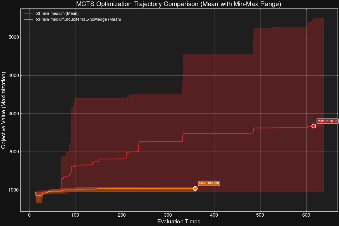
Effect of scale
Contributions of knowledge synthesis
Combining the interpretability of physics with the power of AI
Our Mission: To create transparent AI systems that combine physics-based interpretability with deep learning capabilities
Interpretable AI Approach
The best of both worlds
Input
Physics-Informed
AI Algorithm
(High interpretability)
Output
Example: Our Approach
(In Preparation)
AI Model
Physics
Knowledge
Traditional Physics Approach
Input
Human-Designed Algorithm
(Based on human insight)
Output
Example: Matched Filtering, linear regression
Black-Box AI Approach
Input
AI Model
(Low interpretability)
Output
Examples: CNN, AlphaGo, DINGO
Data/
Experience
Data/
Experience
Interpretable Gravitational Wave Data Analysis with DL and LLMs
Key Insights from Our Journey
The Critical Role of Interpretability
Algorithm interpretability provides multiple essential benefits:
The future of gravitational wave science lies at the intersection of traditional physics-inspired methods and interpretable AI approaches, creating a new paradigm for reliable scientific discovery.
for _ in range(num_of_audiences):
    print('Thank you for your attention! 🙏')
hewang@ucas.ac.cn
Interpretable Gravitational Wave Data Analysis with DL and LLMs
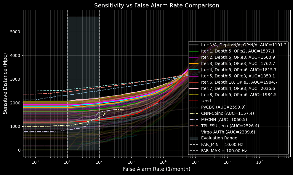
Preliminary Results (February 2025)
Optimization Progress & Algorithm Diversity
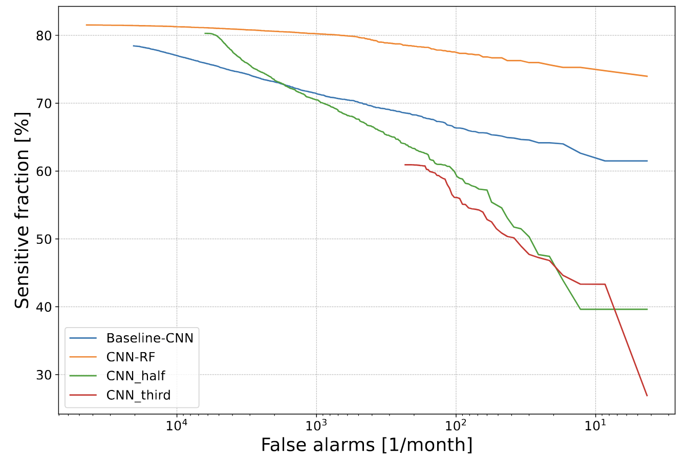
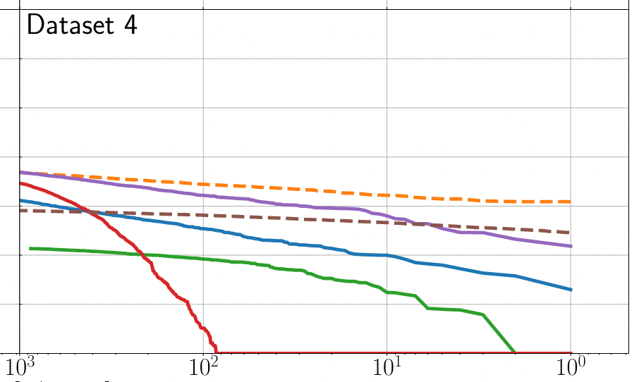
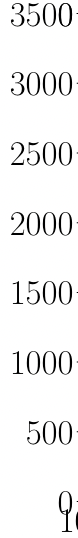
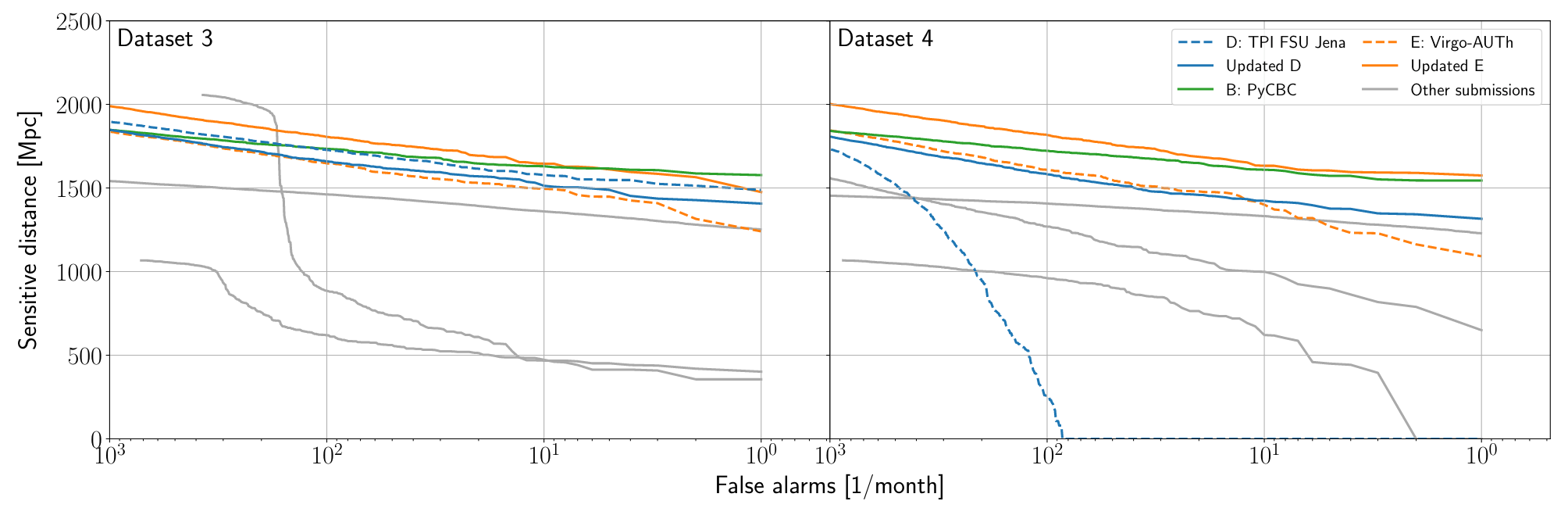
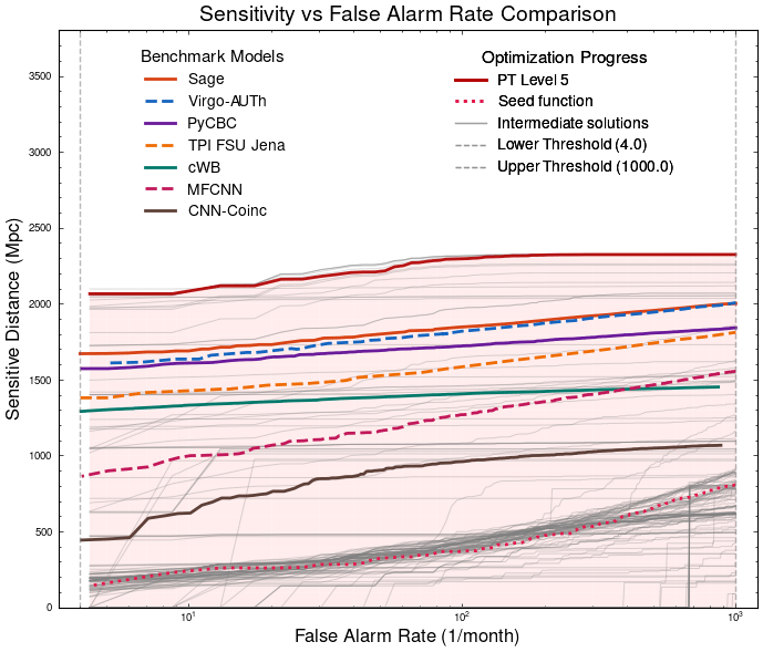
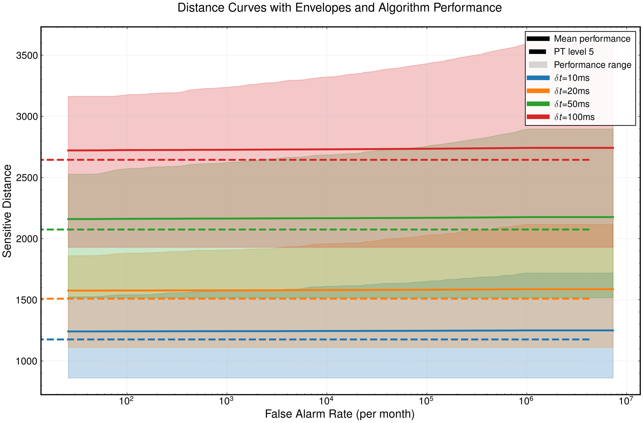
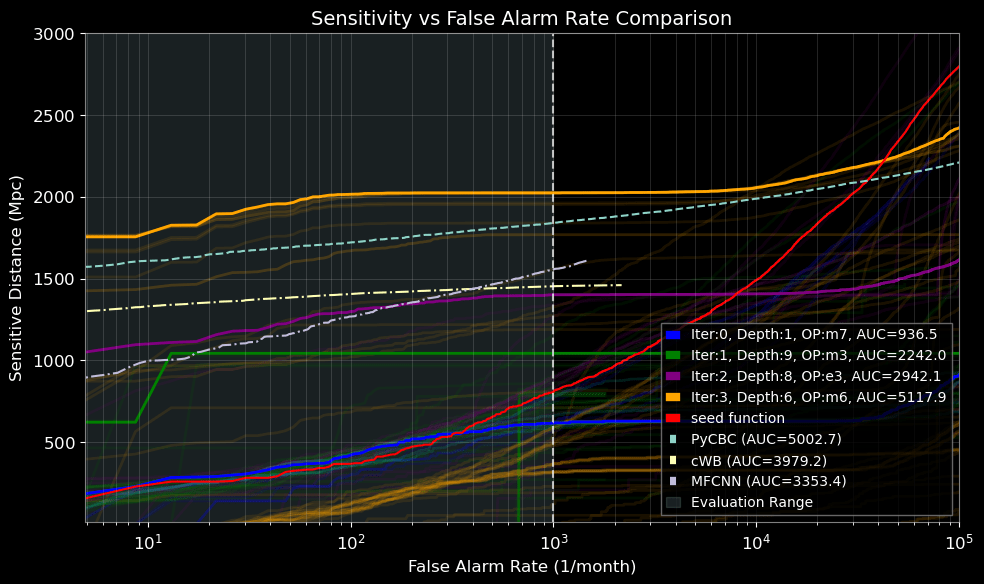
Sensitivity vs False Alarm Rate
Optimization Target: Maximizing Area Under Curve (AUC) in the 1-1000 false alarms per-month range, balancing detection sensitivity and false alarm rates across algorithm generations
Our framework (agent-based LLMs) can effectively optimize complex algorithms and guide iterative development along specified optimization directions, achieving targeted performance improvements in GW detection
Pipeline Workflow
Interpretable Gravitational Wave Data Analysis with DL and LLMs
Preliminary Results (February 2025)
Optimization Progress & Algorithm Diversity
Pipeline Workflow
This pipeline combines adaptive PSD whitening and multi-band spectral coherence computation with a noise floor-aware peak detection and a non-linear timing uncertainty model to enhance gravitational wave signal detection accuracy and robustness. It computes coherent time-frequency metric (with frequency-dependent regularization and entropy-based symmetry enforcement) and validates candidate signals via geometric features and multi-resolution thresholding (including dyadic wavelet analysis).
Integrate asymmetric PSD whitening, extended STFT overlap optimization, chirp-enhanced prominence scaling, multi-channel noise floor refinement, and dynamic timing calibration for improved gravitational wave signal detection.
The pipeline first applies adaptive local parameter control and noise-adaptive statistical regularization\u2014dynamically tuning median filter kernels, whitening gains, and spectral smoothness\u2014to detrend and whiten the dual-channel gravitational wave data, prioritizing robust noise baseline estimation over high-frequency variations. Then, it computes a coherent time-frequency metric (with frequency-dependent regularization and entropy-based symmetry enforcement) and validates candidate signals via geometric features and multi-resolution thresholding (including dyadic wavelet analysis), ultimately outputting candidate trigger GPS times, significance levels, and timing uncertainties.
Optimization Target: Maximizing Area Under Curve (AUC) in the 1-1000 false alarms per-month range, balancing detection sensitivity and false alarm rates across algorithm generations
Interpretable Gravitational Wave Data Analysis with DL and LLMs
Our framework (agent-based LLMs) can effectively optimize complex algorithms and guide iterative development along specified optimization directions, achieving targeted performance improvements in GW detection
Preliminary Results (February 2025)
Sensitivity vs False Alarm Rate
Our framework (agent-based LLMs) can effectively optimize complex algorithms and guide iterative development along specified optimization directions, achieving targeted performance improvements in GW detection
Optimization Target: Maximizing Area Under Curve (AUC) in the 1-1000 false alarms per-month range, balancing detection sensitivity and false alarm rates across algorithm generations
PyCBC (linear-like)
cWB (linear-like)
Simple non-linear filters
CNN-like (highly non-linear)
Interpretable Gravitational Wave Data Analysis with DL and LLMs
Q1: Can LLMs truly generate novel content beyond their training data?
Q2: Why can LLMs perform reasoning in ways that remain imperceptible to us?
Interpretable Gravitational Wave Data Analysis with DL and LLMs
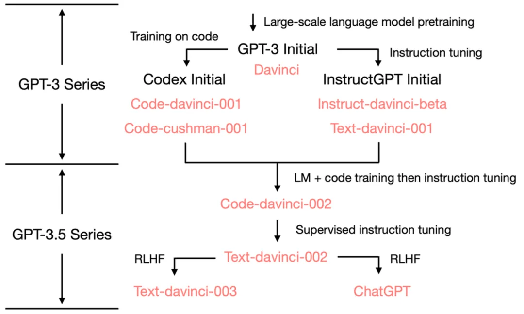
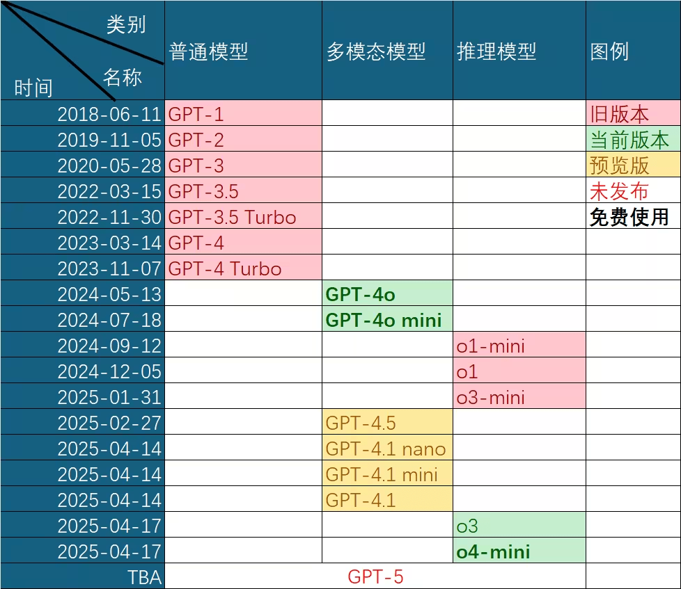
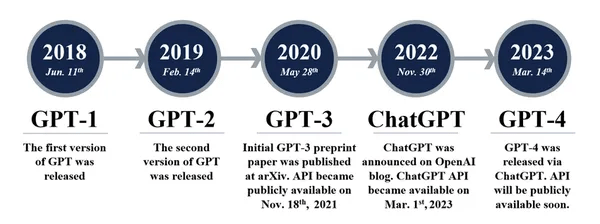
Evolution of GPT Capabilities
A careful examination of GPT-3.5's capabilities reveals the origins of its emergent abilities:
GPT-3.5 series [Source: University of Edinburgh, Allen Institute for AI]
GPT-3 (2020)
ChatGPT (2022)
Magic: Code + Text
Interpretable Gravitational Wave Data Analysis with DL and LLMs
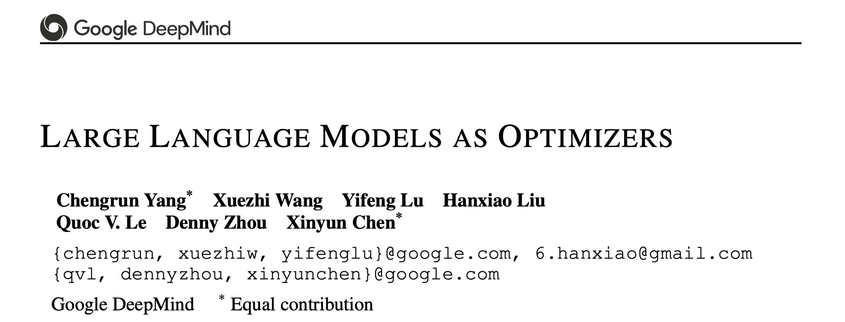
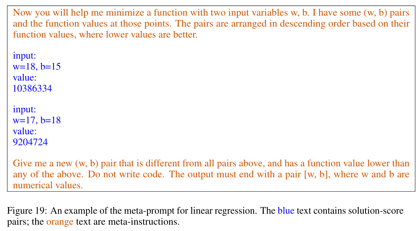
Recent research demonstrates that LLMs can solve complex optimization problems through carefully engineered prompts. DeepMind's OPRO (Optimization by PROmpting) approach showcases how LLMs can generate increasingly refined solutions through iterative prompting techniques.
OPRO: Optimization by PROmpting
Example: Least squares optimization through prompt engineering
arXiv:2309.03409 [cs.NE]
Two Directions of LLM-based Optimization
arXiv:2405.10098 [cs.NE]
LLMs can generate high-quality solutions to optimization problems without specialized training
Interpretable Gravitational Wave Data Analysis with DL and LLMs
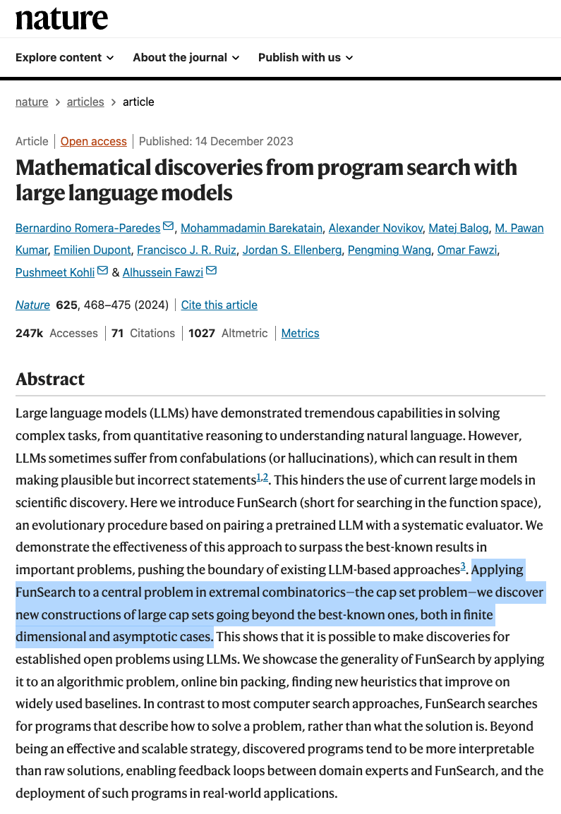
The Interpolation Theory
LLMs' ability to generate novel responses from few examples is increasingly understood as manifold interpolation rather than mere memorization:
The theory suggests that in-context learning is not "learning" in the traditional sense, but rather a form of implicit conditioning on the manifold of learned representations.
Representation Space Interpolation
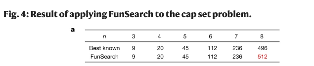
Real-world Case: FunSearch (Nature, 2023)
Interpretable Gravitational Wave Data Analysis with DL and LLMs
Q1: Can LLMs truly generate novel content beyond their training data?
Q2: Why can LLMs perform reasoning in ways that remain imperceptible to us?
Interpretable Gravitational Wave Data Analysis with DL and LLMs
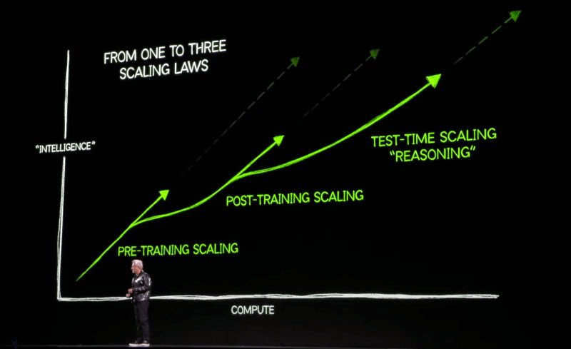
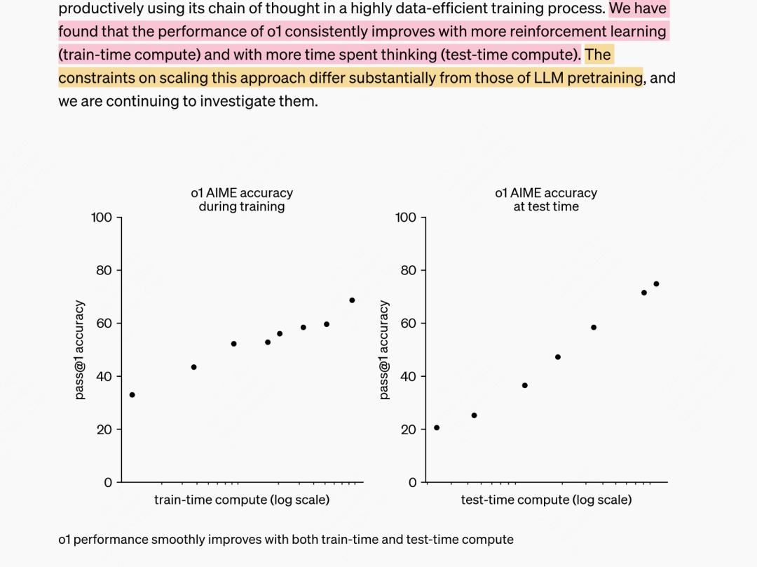
📄 Google DeepMind: "Scaling LLM Test-Time Compute Optimally" (arXiv:2408.03314)
🔗 OpenAI: Learning to Reason with LLMs
Iterative refinement during inference dramatically improves reasoning capabilities without increasing model size or retraining
Performance improvements with test-time compute scaling
From pre-training to test-time:
Three scaling regimes
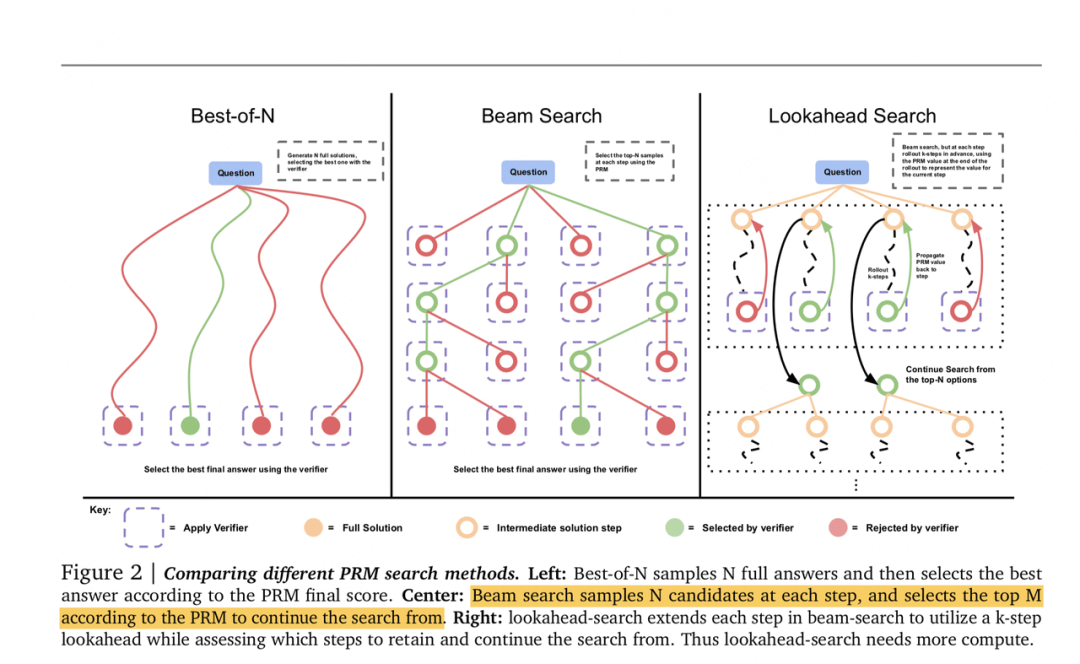
Different search methods for iterative reasoning
Interpretable Gravitational Wave Data Analysis with DL and LLMs
Combining the interpretability of physics with the power of AI
Our Mission: To create transparent AI systems that combine physics-based interpretability with deep learning capabilities
Interpretable AI Approach
The best of both worlds
Input
Physics-Informed
Algorithm
(High interpretability)
Output
Example: Our Approach
(In Preparation)
AI Model
Physics
Knowledge
Traditional Physics Approach
Input
Human-Designed Algorithm
(Based on human insight)
Output
Example: Matched Filtering, linear regression
Black-Box AI Approach
Input
AI Model
(Low interpretability)
Output
Examples: CNN, AlphaGo, DINGO
Data/
Experience
Data/
Experience
Interpretable Gravitational Wave Data Analysis with DL and LLMs
Key Insights from Our Journey
The Critical Role of Interpretability
Algorithm interpretability provides multiple essential benefits:
The future of gravitational wave science lies at the intersection of traditional physics-inspired methods and interpretable AI approaches, creating a new paradigm for reliable scientific discovery.
for _ in range(num_of_audiences):
    print('Thank you for your attention! 🙏')
hewang@ucas.ac.cn
Interpretable Gravitational Wave Data Analysis with DL and LLMs
Q1: Can LLMs truly generate novel content beyond their training data?
Q2: Why can LLMs perform reasoning in ways that remain imperceptible to us?
Q3: Does our framework require special design to achieve these capabilities?
Interpretable Gravitational Wave Data Analysis with DL and LLMs
Given the interpretability challenges we've explored,
how might we advance GW detection and parameter estimation while maintaining scientific rigor?
The Interpolation Theory
LLMs' ability to generate novel responses from few examples is increasingly understood as manifold interpolation rather than mere memorization:
The theory suggests that in-context learning is not "learning" in the traditional sense, but rather a form of implicit conditioning on the manifold of learned representations.
Representation Space Interpolation
Key Literature
The Interpolation Theory
LLMs' ability to generate novel responses from few examples is increasingly understood as manifold interpolation rather than mere memorization:
The theory suggests that in-context learning is not "learning" in the traditional sense, but rather a form of implicit conditioning on the manifold of learned representations.
Representation Space Interpolation
Key Literature on Manifold Interpolation
https://www.lesswrong.com/posts/GADJFwHzNZKg2Ndti/have-llms-generated-novel-insights
https://gowrishankar.info/blog/deep-learning-is-not-as-impressive-as-you-think-its-mere-interpolation/
REWIRING AGI—NEUROSCIENCE IS ALL YOU NEED
What is test-time scaling?
Why LLMs can do the inference/optimation?
How about the theory? (check: 2410.14716)
Why we need MCTS?
Why and How is Evoluation theory in Opt area?
Add computational complexity analysis
借用流浪地球的台词?
借用流浪地球的台词?
Drawbacks and limitations:
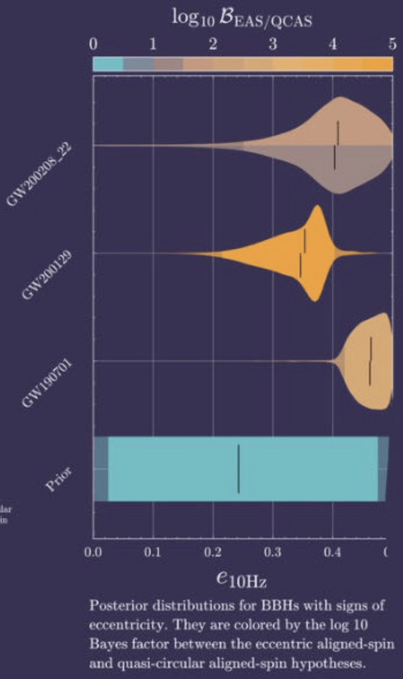
好好先review一下:eccentricity using DINGO; AreaGW
自己实验的OPRO效果
好好先review一下:eccentricity using DINGO; AreaGW
逐层递进深刻的reflection
自己实验的符号回归
Mathematics of HAD ?
import numpy as np
import scipy.signal as signal
def pipeline_v1(strain_h1: np.ndarray, strain_l1: np.ndarray, times: np.ndarray) -> tuple[np.ndarray, np.ndarray, np.ndarray]:
    def data_conditioning(strain_h1: np.ndarray, strain_l1: np.ndarray, times: np.ndarray) -> tuple[np.ndarray, np.ndarray, np.ndarray]:
        window_length = 4096
        dt = times[1] - times[0]
        fs = 1.0 / dt

        def whiten_strain(strain):
            strain_zeromean = strain - np.mean(strain)
            freqs, psd = signal.welch(strain_zeromean, fs=fs, nperseg=window_length,
                                       window='hann', noverlap=window_length//2)
            smoothed_psd = np.convolve(psd, np.ones(32) / 32, mode='same')
            smoothed_psd = np.maximum(smoothed_psd, np.finfo(float).tiny)
            white_fft = np.fft.rfft(strain_zeromean) / np.sqrt(np.interp(np.fft.rfftfreq(len(strain_zeromean), d=dt), freqs, smoothed_psd))
            return np.fft.irfft(white_fft)

        whitened_h1 = whiten_strain(strain_h1)
        whitened_l1 = whiten_strain(strain_l1)

        return whitened_h1, whitened_l1, times

    def compute_metric_series(h1_data: np.ndarray, l1_data: np.ndarray, time_series: np.ndarray) -> tuple[np.ndarray, np.ndarray]:
        fs = 1 / (time_series[1] - time_series[0])
        f_h1, t_h1, Sxx_h1 = signal.spectrogram(h1_data, fs=fs, nperseg=256, noverlap=128, mode='magnitude', detrend=False)
        f_l1, t_l1, Sxx_l1 = signal.spectrogram(l1_data, fs=fs, nperseg=256, noverlap=128, mode='magnitude', detrend=False)
        tf_metric = np.mean((Sxx_h1**2 + Sxx_l1**2) / 2, axis=0)
        gps_mid_time = time_series[0] + (time_series[-1] - time_series[0]) / 2
        metric_times = gps_mid_time + (t_h1 - t_h1[-1] / 2)

        return tf_metric, metric_times

    def calculate_statistics(tf_metric, t_h1):
        background_level = np.median(tf_metric)
        peaks, _ = signal.find_peaks(tf_metric, height=background_level * 1.0, distance=2, prominence=background_level * 0.3)
        peak_times = t_h1[peaks]
        peak_heights = tf_metric[peaks]
        peak_deltat = np.full(len(peak_times), 10.0)  # Fixed uncertainty value
        return peak_times, peak_heights, peak_deltat

    whitened_h1, whitened_l1, data_times = data_conditioning(strain_h1, strain_l1, times)
    tf_metric, metric_times = compute_metric_series(whitened_h1, whitened_l1, data_times)
    peak_times, peak_heights, peak_deltat = calculate_statistics(tf_metric, metric_times)

    return peak_times, peak_heights, peak_deltat
Function Role in Framework
Pipeline Workflow
Input: H1 and L1 detector strains, time array | Output: Event times, significance values, and time uncertainties
Preliminary Results (February 2025)
Prompt Structure for Algorithm Evolution
This template guides the LLM to generate optimized gravitational wave detection algorithms by learning from comparative examples.
Key Components:
One Prompt Template for MLGWSC1 Algorithm Synthesis
You are an expert in gravitational wave signal detection algorithms. Your task is to design heuristics that can effectively solve optimization problems.

{prompt_task}

I have analyzed two algorithms and provided a reflection on their differences.

[Worse code]
{worse_code}

[Better code]
{better_code}

[Reflection]
{reflection}

Based on this reflection, please write an improved algorithm according to the reflection.
First, describe the design idea and main steps of your algorithm in one sentence. The description must be inside a brace outside the code implementation. Next, implement it in Python as a function named '{func_name}'.
This function should accept {input_count} input(s): {joined_inputs}. The function should return {output_count} output(s): {joined_outputs}.
{inout_inf} {other_inf}

Do not give additional explanations.
Preliminary Results (February 2025)
Preliminary Results (February 2025)
Optimization Progress & Algorithm Diversity
Sensitivity vs False Alarm Rate
Optimization Target: Maximizing Area Under Curve (AUC) in the 10-100Hz frequency range, balancing detection sensitivity and false alarm rates across algorithm generations
Optimization Target: Maximizing Area Under Curve (AUC) in the 10-100Hz frequency range, balancing detection sensitivity and false alarm rates across algorithm generations
Preliminary Results (February 2025)
This pipeline combines adaptive PSD whitening and multi-band spectral coherence computation with a noise floor-aware peak detection and a non-linear timing uncertainty model to enhance gravitational wave signal detection accuracy and robustness.
Integrate asymmetric PSD whitening, extended STFT overlap optimization, chirp-enhanced prominence scaling, multi-channel noise floor refinement, and dynamic timing calibration for improved gravitational wave signal detection.
Optimization Target: Maximizing Area Under Curve (AUC) in the 10-100Hz frequency range, balancing detection sensitivity and false alarm rates across algorithm generations
Optimization Progress & Algorithm Diversity
Preliminary Results (February 2025)
The framework (LLMs) can effectively optimize complex algorithms and guide iterative development along specified optimization directions, achieving targeted performance improvements in GW detection
Preliminary Results (February 2025)
Sensitivity vs False Alarm Rate
PyCBC
CNN-like
Simple non-linear filter
Key Finding: Our framework demonstrates potential to optimize highly interpretable and scalable non-linear algorithm pipelines that achieve performance comparable to traditional matched filtering techniques.
Traditional Physics Approach
Input
Human-Designed Algorithm
(Based on human insight)
Output
Example: Matched Filtering
Black-Box AI Approach
Input
AI Model
(Low interpretability)
Output
Examples: CNN, AlphaGo
Interpretable AI Approach
Input
Optimized
Algorithm
(High interpretability)
Output
Example: OURS (on-going)
The Future: Combining traditional physics knowledge with LLM-optimized algorithms for transparent, reliable scientific discovery
Data/
Experience
Data/
Experience
AI Model
Data/
Experience
Key Insights from Our Journey
The Critical Role of Interpretability
Algorithm interpretability provides multiple essential benefits:
The future of gravitational wave science lies at the intersection of traditional physics-inspired methods and interpretable AI approaches, creating a new paradigm for reliable scientific discovery.
for _ in range(num_of_audiences):
    print('Thank you for your attention! 🙏')
hewang@ucas.ac.cn
By He Wang
2025/05/26 10:15-10:35 @SHAO KIW-12


