


He Wang PRO
Knowledge increases by sharing but not by saving.
Lecturer:He Wang (王赫)
2025/11/13 @FQCP2025
ICTP-AP, UCAS
Who Am I
— A quick intro and how I got into this field
What Is Machine Learning?
— The basics and why it matters
Deep Learning: When Machines Start to See and Think
— From neural networks to powerful representations
Gravitational Waves Meet Machine Learning
— How ML is reshaping data analysis in GW astronomy
Let’s Get Practical: Searching for Gravitational Waves
— A hands-on look at applying ML in real GW searches
LLMs for Gravitational Waves: My Ongoing Work
— Towards automated and interpretable scientific discovery
# Who am I
He Wang received his Ph.D. in Theoretical Physics from Beijing Normal University in 2020. He is currently an Associate Researcher (E-Series) at the ICTP-AP, UCAS. After completing his Ph.D., he conducted postdoctoral research at the ITP-CAS, the Peng Cheng National Laboratory (as a visiting scholar), and UCAS.
He serves as the Co-chair of the LVK Machine Learning Algorithms Group, a Core Member of the LISA Consortium, and a Youth Data Scientist at the National Astronomical Data Center (NADC). As a core contributor to China’s Taiji Program for Space Gravitational Wave Detection, his work focuses on scientific data analysis and algorithmic development.
Machine learning and GW data analysis @TianQin Center
Who Am I
— A quick intro and how I got into this field
What Is Machine Learning?
— The basics and why it matters
Deep Learning: When Machines Start to See and Think
— From neural networks to powerful representations
Gravitational Waves Meet Machine Learning
— How ML is reshaping data analysis in GW astronomy
Let’s Get Practical: Searching for Gravitational Waves
— A hands-on look at applying ML in real GW searches
LLMs for Gravitational Waves: My Ongoing Work
— Towards automated and interpretable scientific discovery
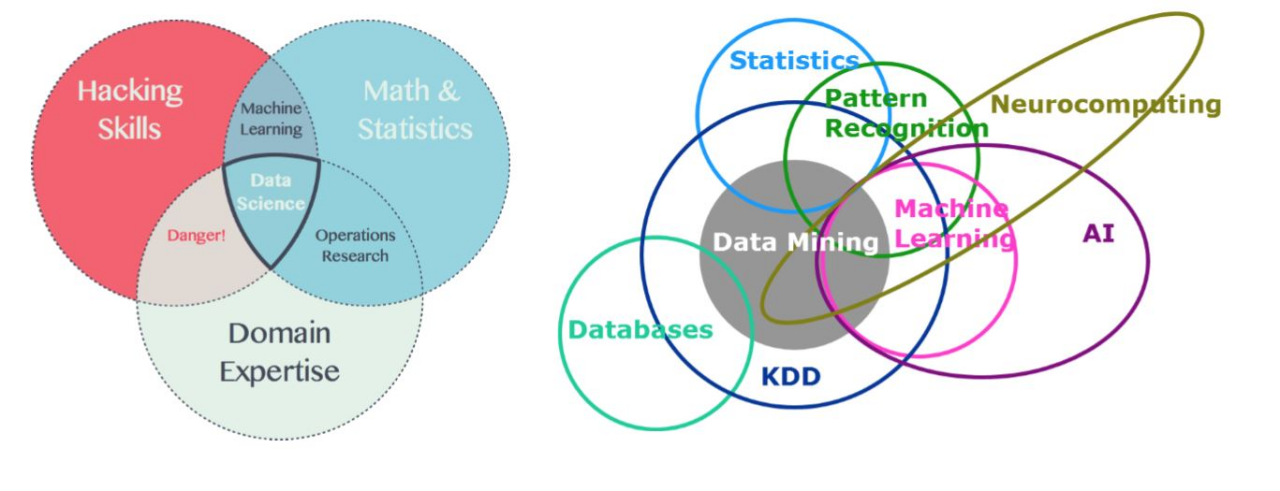
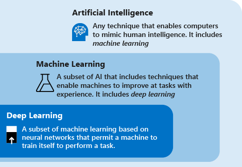
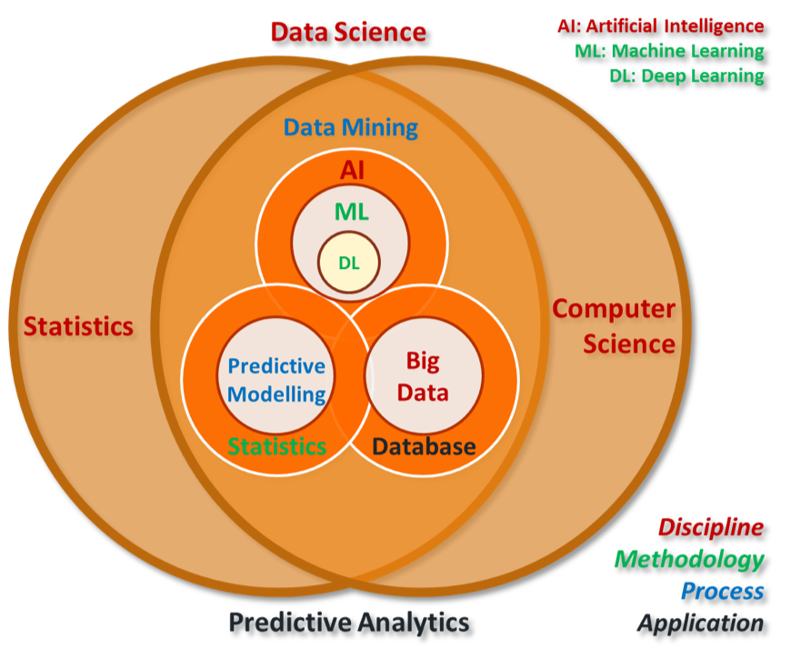
# GW: ML
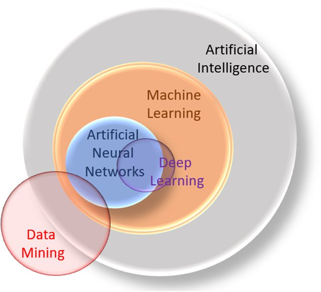
Machine Learning
A major branch of Artificial Intelligence (AI) focused on improving algorithmic performance through learning from experience.
Typical models include Linear Regression, Decision Trees, Support Vector Machines (SVMs), and Markov Chain Monte Carlo (MCMC) methods.
Deep Learning
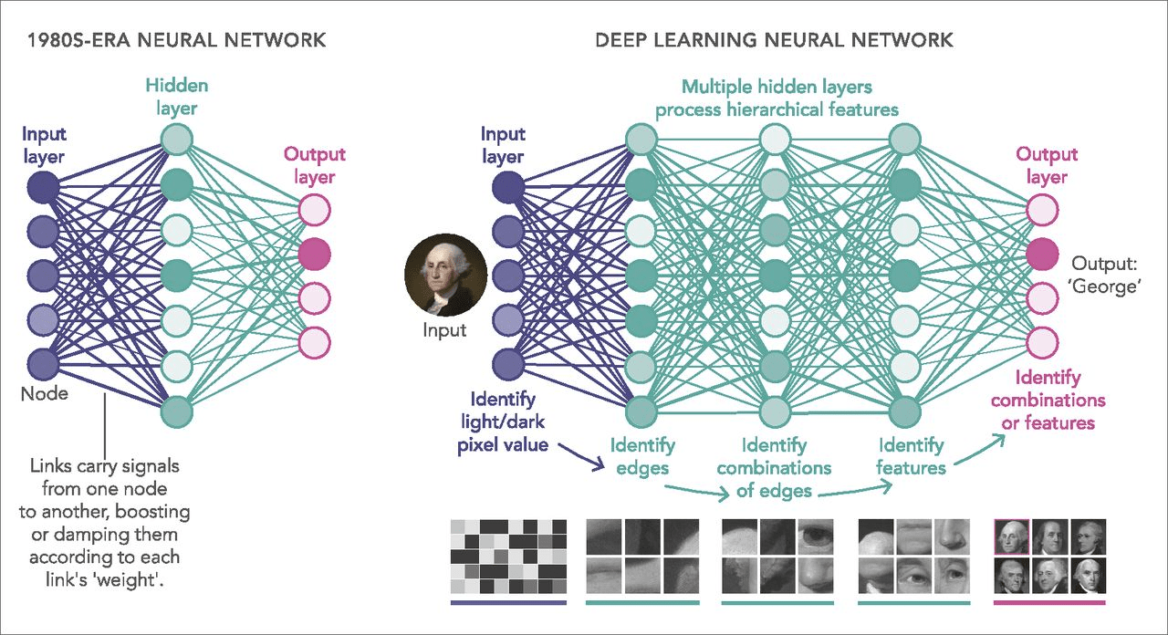
A specialized subfield of machine learning that uses neural networks to automatically extract features from data.
Deep neural networks serve as universal function approximators, capable of modeling complex nonlinear mappings.
Key characteristics: end-to-end learning, data-driven, and over-parameterized architectures.
Data-driven approaches: discovering patterns and regularities from data through algorithms and applying them to new data.
Knowledge Discovery in Database, KDD
“机器学习是对能通过经验自动改进的计算机算法的研究。”
Machine Learning is the study of computer algorithms that improve automatically through experience.
“机器学习是用数据或以往的经验,以此优化计算机程序的性能标准。”
Machine learning is programming computers to optimize a performance criterion using example data or past experience.
——Alpaydin (2004)
A computer program is said to learn from experience E with respect to some class of tasks T and performance measure P, if its performance at tasks in T, as measured by P, improves with experience E. ——Tom Mitchell (1997)
# GW: ML
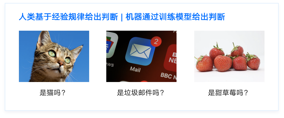
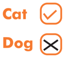
Humans make judgments based on experience —
Machines make judgments by training models on data.
Is it a cat?
Is it a spam?
Is it a sweet
strawberry?
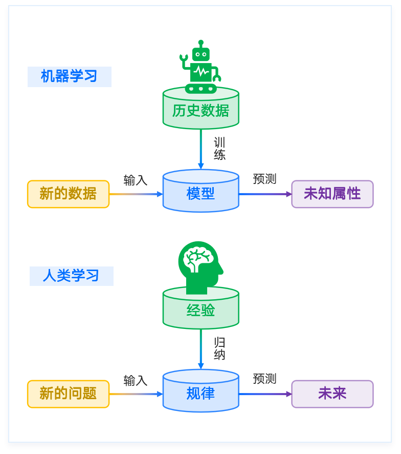
Machine learning
Human learning
experience
data
train
train
input
input
new data
new problem
predict
predict
unknown property
future
# GW: ML
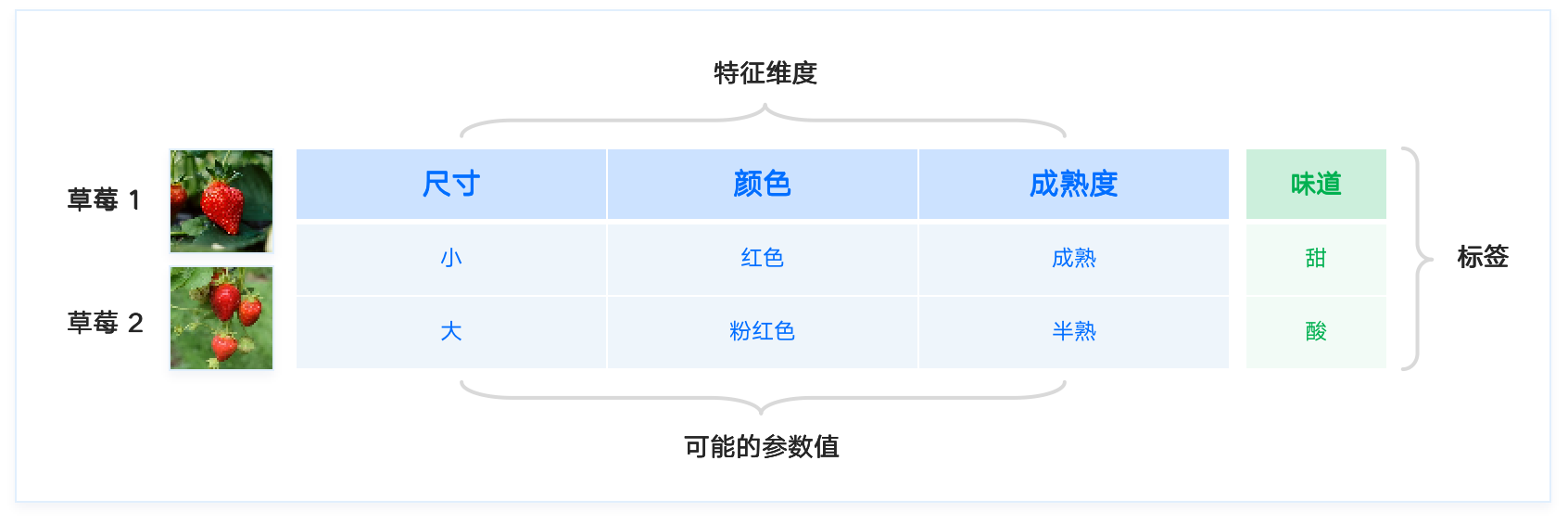
Task [T]: Determine whether a strawberry is sweet.
Machine learning aims to find the mapping between a strawberry’s features (size, color, ripeness, etc.) and its label (sweet or sour).
Feature Dimensions
Strawberry 1
Strawberry 2
Possible Feature Values
Label
Size
Color
Ripeness
Ripe
|
Half-ripe |
Red
Pink
Small
Large
Taste
Sweet
Sour
# GW: ML
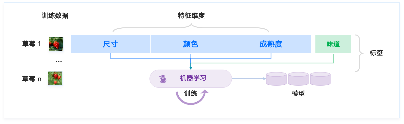
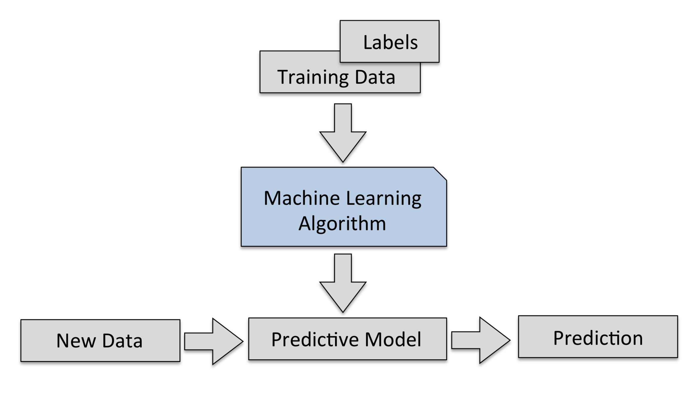
Machine learning aims to discover the relationship between features and labels.
It uses algorithms to automatically analyze a set of training data, learn underlying patterns, and apply them to predict unseen data.
This process of finding patterns and relationships is called training, and the outcome of training is a machine learning model.
Feature Dimensions
Strawberry 1
Strawberry n
Label
Size
Color
Ripeness
ML model
train
Machine Learning
Taste
Training dataset
# GW: ML
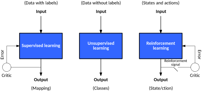
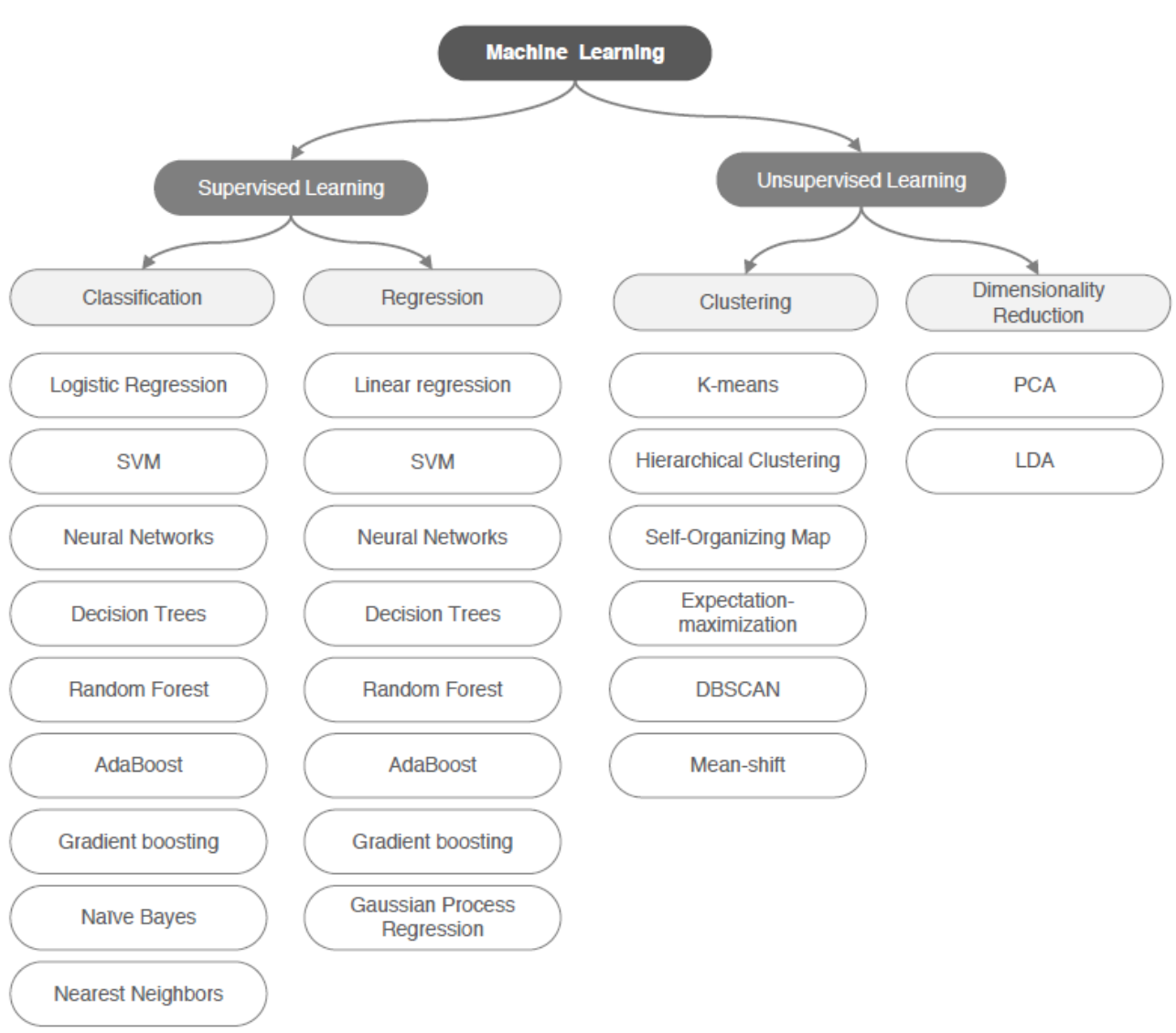
Machine learning models can be broadly categorized based on the presence of labels in training data and how they interact with their environment:
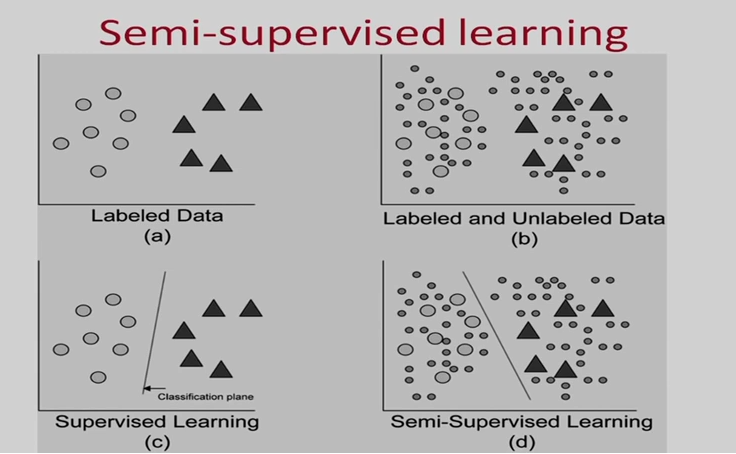
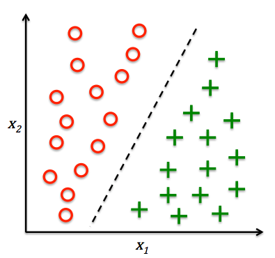
Supervised Learning — learning from labeled data
Unsupervised Learning — discovering structure in unlabeled data
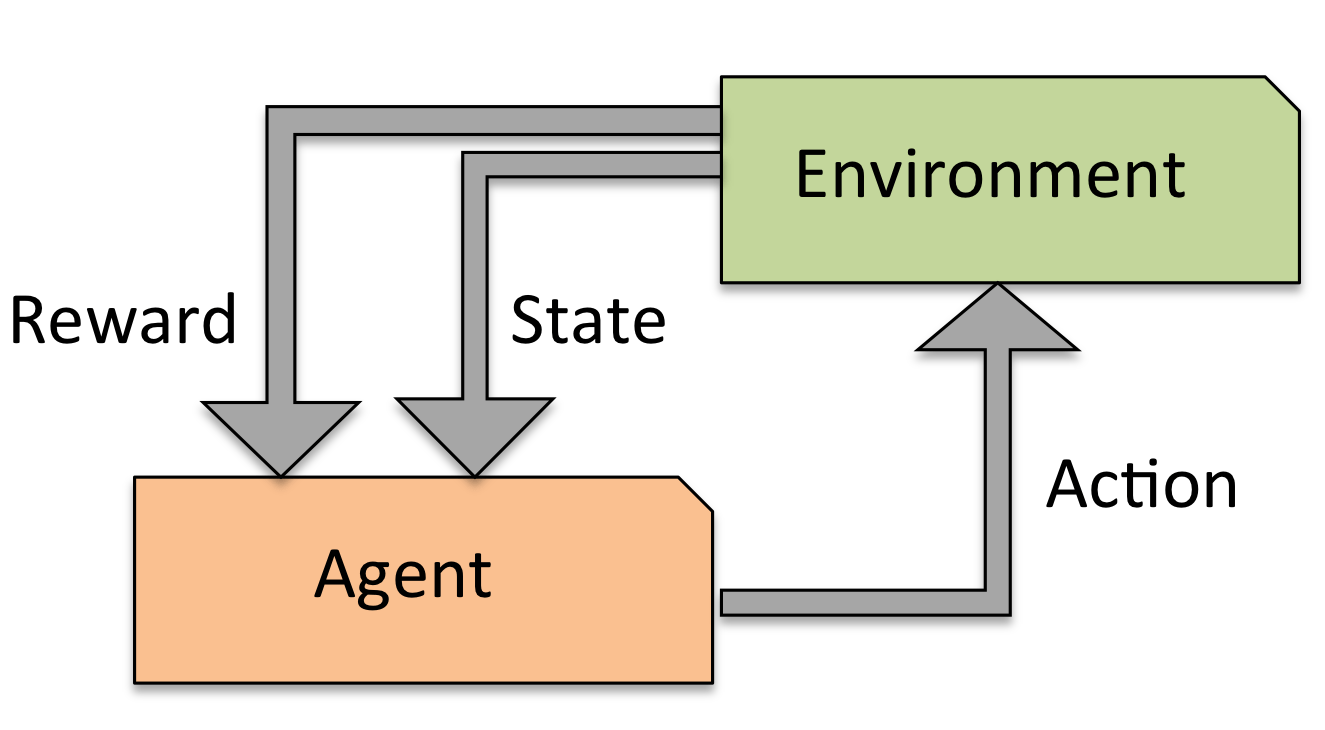
Reinforcement Learning — learning through interaction and feedback from the environment
# GW: ML
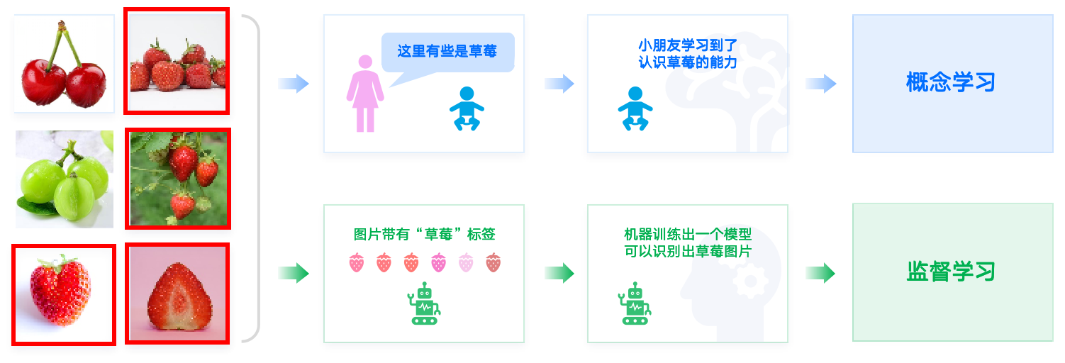
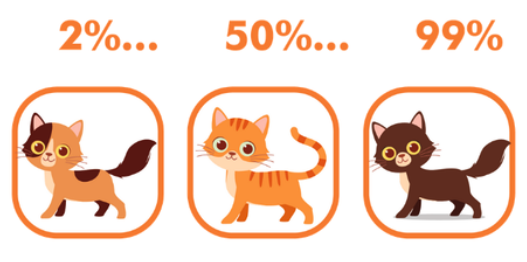
Supervised learning (SL) teaches machines with explicit guidance — the key is that training data are labeled with known outputs (labels).
The goal is for the model, after observing labeled training examples (inputs and expected outputs), to predict the correct output for unseen inputs.
To achieve this, the model must generalize from the observed data in a meaningful way — a process similar to how humans and animals learn concepts from examples, known as concept learning in cognitive science.
Some of these are strawberries.
The child learns to recognize what a strawberry looks like.
Concept Learning
Images are labeled with “strawberry.”
The machine trains a model that can recognize strawberries.
Supervised Learning
# GW: ML
Supervised learning: the key is labeled training data.
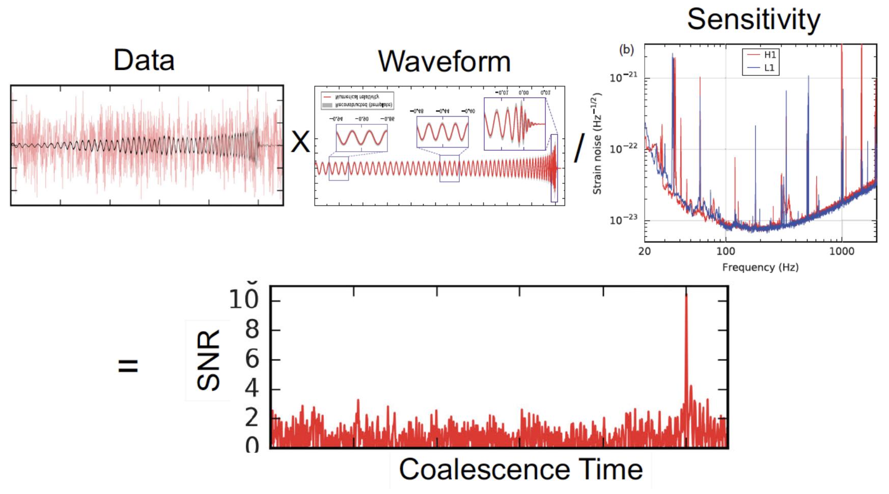
Matched filtering (template-based GW search)
Given a segment of time-series data as input, the detection statistic (the matched-filter signal-to-noise ratio over time) is an output time series.
The core question: Which linear filter (i.e., which template) maximizes that output?
In practice, matched filtering correlates the data with a template waveform and is the optimal linear detector for signals buried in stationary Gaussian noise — it produces the maximum SNR for a given template.
# GW: ML
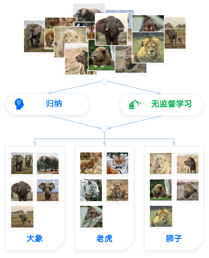
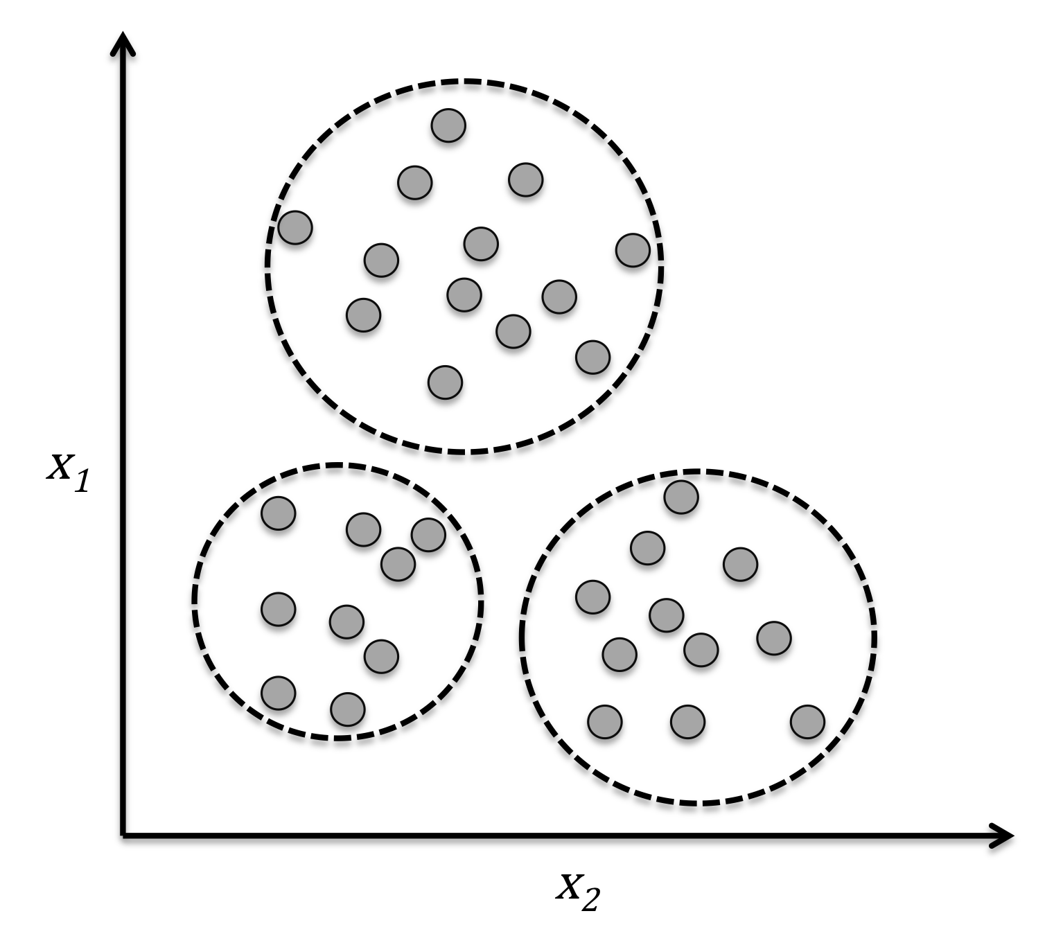
Unsupervised learning (uSL) is a learning process without guidance, where the training data to be learned has no labels.
Machine learning algorithms identify common characteristics in the data through certain methods and group data with shared features together. This process is sometimes referred to as "clustering."
Clustering involves statistically classifying similar objects into different groups or more subsets so that member objects within the same subset share similar attributes.
Unsupervised learning algorithms freely explore the data, and much of what is learned must involve understanding the data itself, rather than applying this understanding to specific tasks. Therefore, mastering unsupervised learning is essential on the path to general intelligence.
The process of unsupervised learning is similar to the human process of inductive learning.
Unsupervised Learning
Induction
Elephant
Tiger
Lion
# GW: ML
Unsupervised learning (uSL) is a learning process without guidance, where the training data to be learned has no labels.
Machine learning algorithms identify common characteristics in the data through certain methods and group data with shared features together. This process is sometimes referred to as "clustering."
Clustering involves statistically classifying similar objects into different groups or more subsets so that member objects within the same subset share similar attributes.
Unsupervised learning algorithms freely explore the data, and much of what is learned must involve understanding the data itself, rather than applying this understanding to specific tasks. Therefore, mastering unsupervised learning is essential on the path to general intelligence.
The process of unsupervised learning is similar to the human process of inductive learning.
# GW: ML
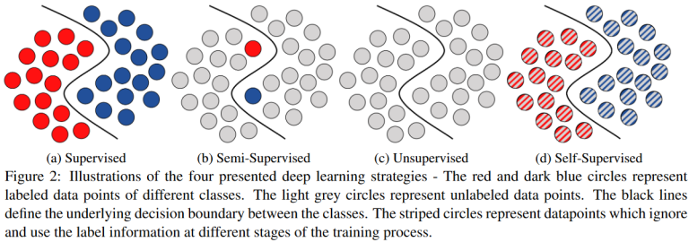
Semi-Supervised Learning (半监督学习)
Self-Supervised Learning (自监督学习)
...
2002.08721
# GW: ML
Prediction Based on Supervised Learning
Classification Tasks
(Predicting Different Categories)
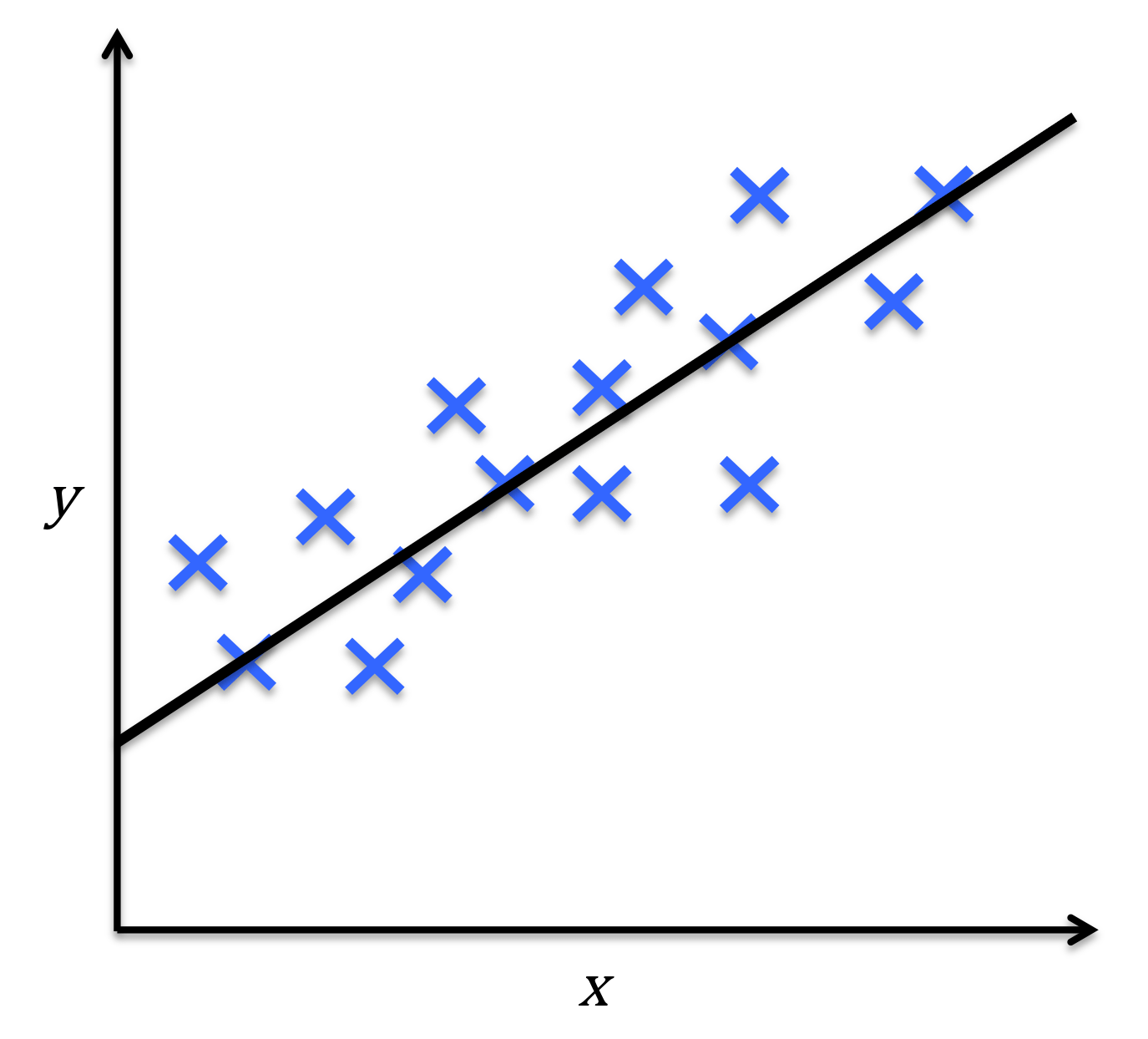
Regression Problems (Predicting Continuous Values)
Unsupervised Learning: Extracting Patterns from Unlabeled Data
Use clustering to discover subgroups.
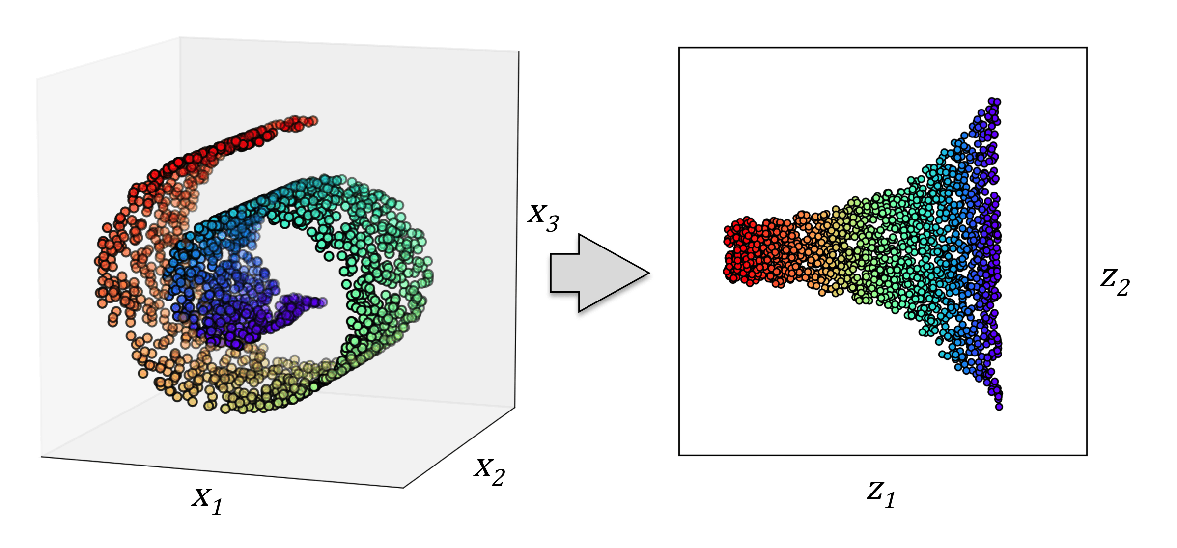
Dimensionality Reduction
Based on the features extracted from data samples, determine which of a finite number of categories they belong to.
Based on the features extracted from data samples, predict continuous value outcomes.
Based on the features extracted from data samples, mine association patterns in the data.
Discover hidden patterns and structures in the data.
# GW: ML
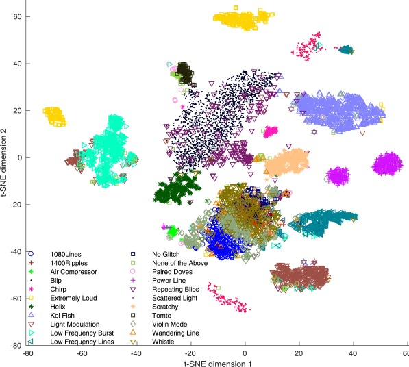
TSNE
UMAP
Based on labels
# GW: ML
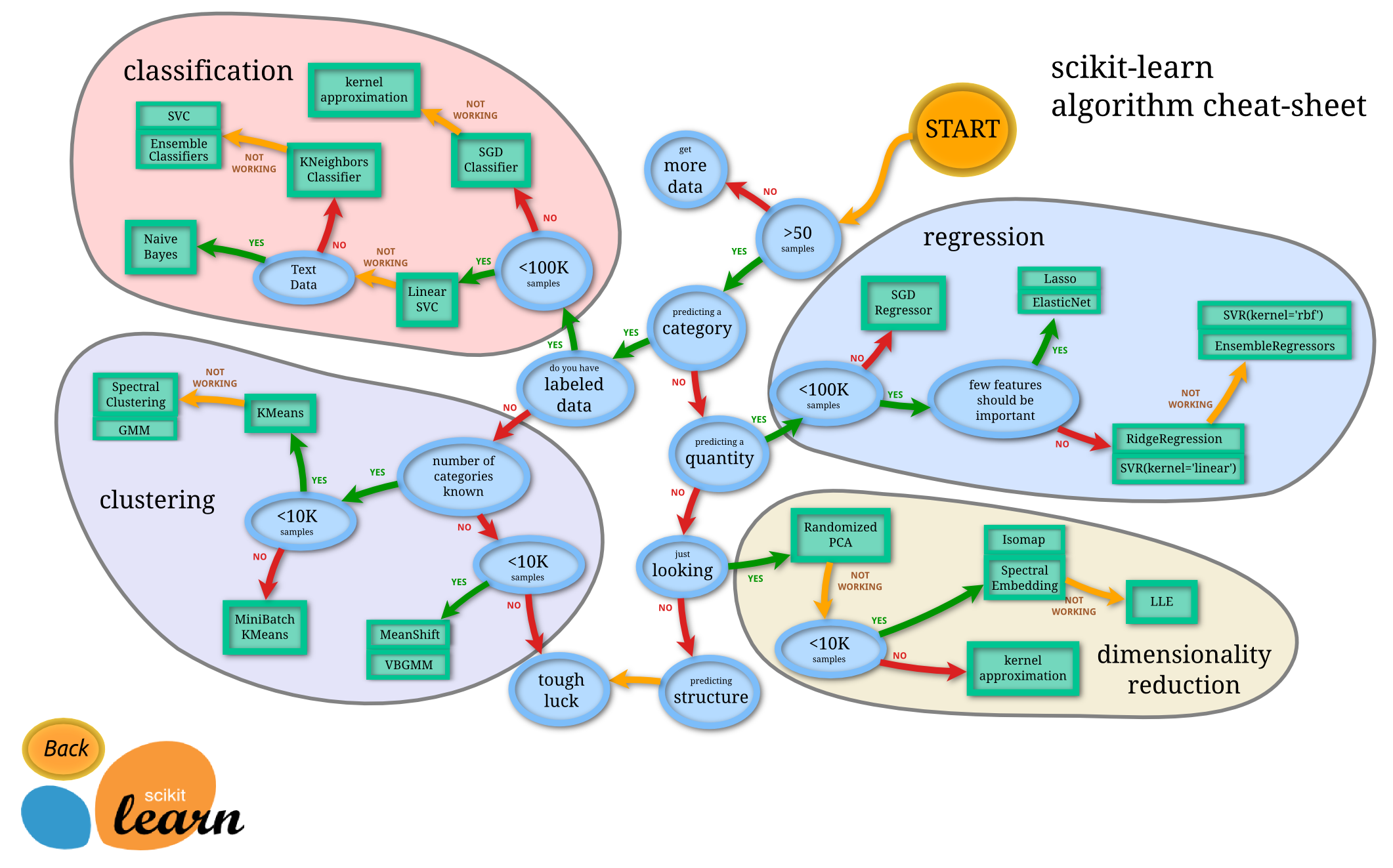
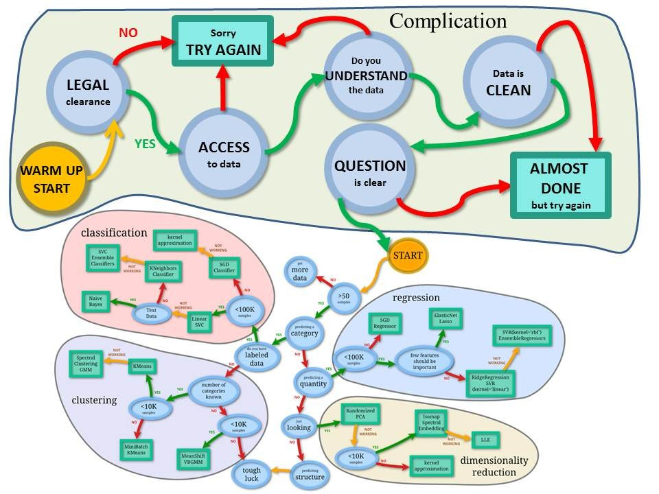
The blue circle contains the judgment criteria, and the green box contains the selectable algorithms. You can find your own operational path based on your data characteristics and task objectives, and just take it step by step.
# GW: ML
# GW: ML
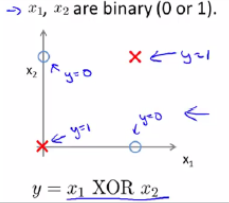
x
y
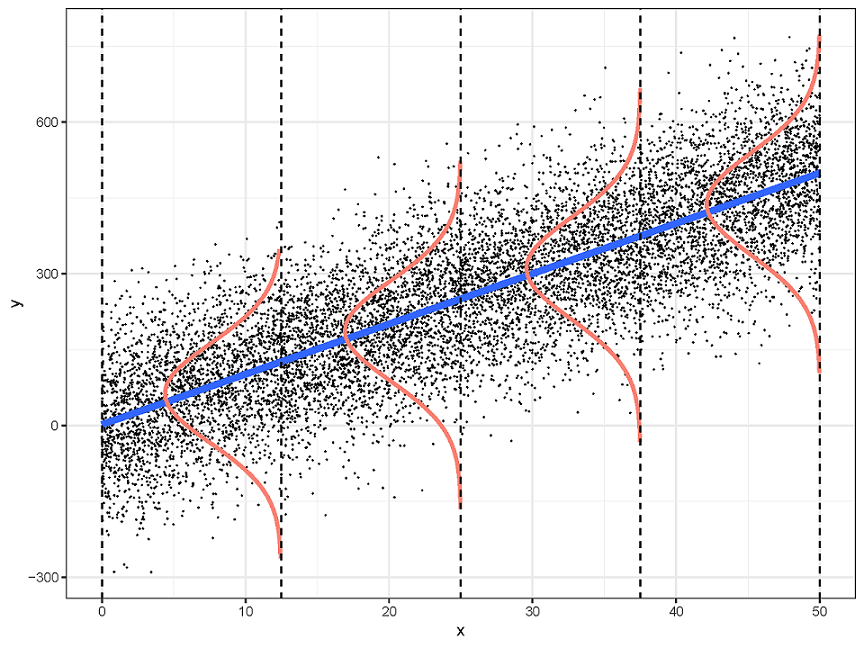
y=mx+b
Conditional Probability \(P(Y|X)\) follows a Gaussian distribution
Linear Regression
Classification by Data Distribution: Parametric vs. Non-Parametric Models
Here, “parametric” does not refer to the parameters within a model, but rather to the parameters of the data distribution itself.
Parametric Models:
Assume a specific form for the data distribution
The underlying data patterns or mappings can be described using a finite and fixed set of model parameters.
Examples: Linear/Logistic Regression, Perceptron, K-Means Clustering
# GW: ML
x
y
y=mx+b
Conditional Probability \(P(Y|X)\) follows a Gaussian distribution
Linear Regression
Classification by Data Distribution: Parametric vs. Non-Parametric Models
Here, “parametric” does not refer to the parameters within a model, but rather to the parameters of the data distribution itself.
Parametric Models:
Assume a specific form for the data distribution
The underlying data patterns or mappings can be described using a finite and fixed set of model parameters.
Examples: Linear/Logistic Regression, Perceptron, K-Means Clustering
Note: In some cases, the data may not provide enough information to assume a prior distribution, or the problem itself may not exhibit any clear distributional characteristics.
# GW: ML
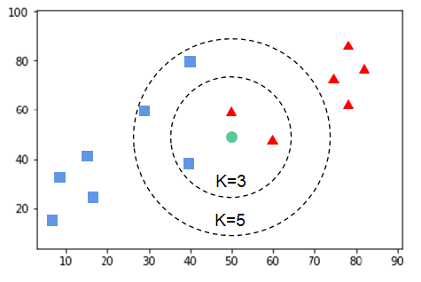
Non-Parametric Models:
Make no assumptions about the form of the data distribution; all statistical properties are derived directly from the data.
Typically have much higher spatial and temporal complexity than parametric models.
Are data-adaptive — the model parameters change dynamically with the samples.
x
y
y=mx+b
Conditional Probability \(P(Y|X)\) follows a Gaussian distribution
Linear Regression
K-Nearest Neighbors
Classification by Data Distribution: Parametric vs. Non-Parametric Models
Here, “parametric” does not refer to the parameters within a model, but rather to the parameters of the data distribution itself.
Parametric Models:
Assume a specific form for the data distribution
The underlying data patterns or mappings can be described using a finite and fixed set of model parameters.
Examples: Linear/Logistic Regression, Perceptron, K-Means Clustering
Examples: Random Forest, Naive Bayes, SVM, Neural Networks
Note: In some cases, the data may not provide enough information to assume a prior distribution, or the problem itself may not exhibit any clear distributional characteristics.
Who Am I
— A quick intro and how I got into this field
What Is Machine Learning?
— The basics and why it matters
Deep Learning: When Machines Start to See and Think
— From neural networks to powerful representations
Gravitational Waves Meet Machine Learning
— How ML is reshaping data analysis in GW astronomy
Let’s Get Practical: Searching for Gravitational Waves
— A hands-on look at applying ML in real GW searches
LLMs for Gravitational Waves: My Ongoing Work
— Towards automated and interpretable scientific discovery
# GW: DL
Machine Learning: A key branch of artificial intelligence and an interdisciplinary field
Data-Driven: Discovering patterns and regularities from data through algorithms and applying them to new data
Knowledge Discovery in Database, KDD
# GW: DL
# GW: DL
# GW: DL
# GW: DL
SVM (support vector machines)
# GW: DL
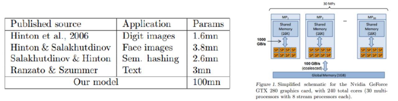
Rajat Raina & Andrew Y. Ng. (ICML09)
(~1970)
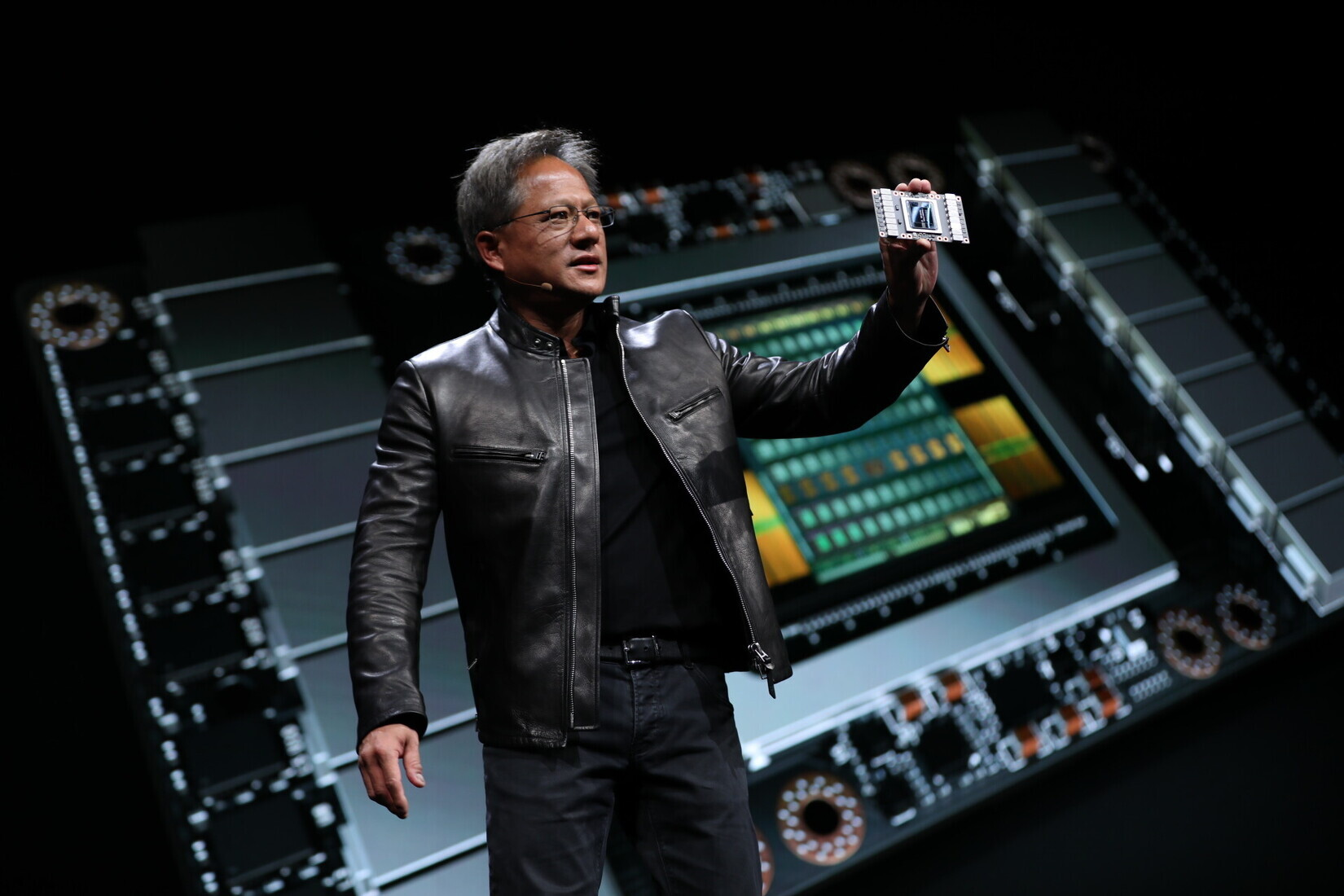
Jen-Hsun Huang.
GPU for DL (~2010)
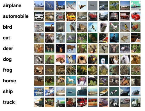
Fei-Fei Li (ILSVRC2010)
# GW: DL
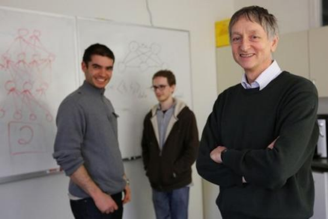
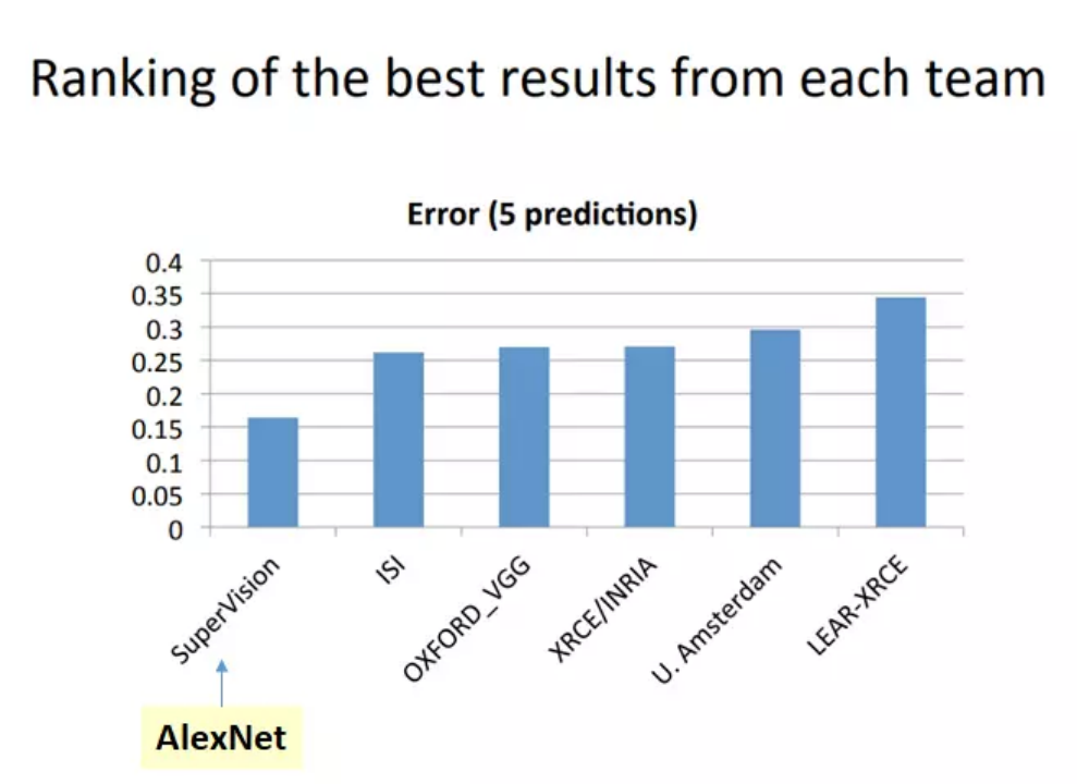
Alex Krizhevsky
Ilya Sutskever
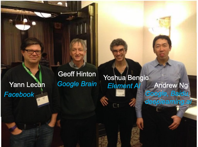
Geoffrey Hinton
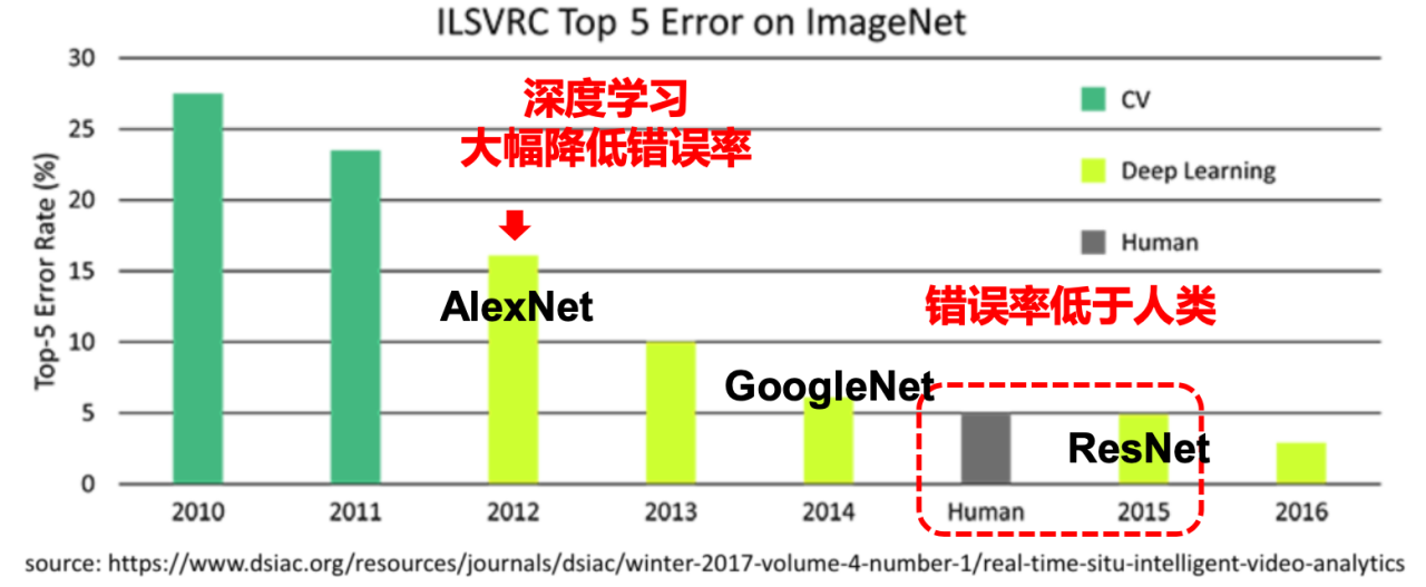
Deep learning
dramatically reduced error rates.
Error rate below human level
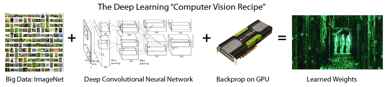
# GW: DL
Big Data (Massive scale)
Algorithms
(Neural Networks)
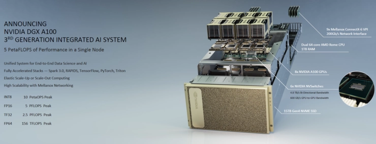
Computing Power (GPU Hardware)
Artificial Intelligence
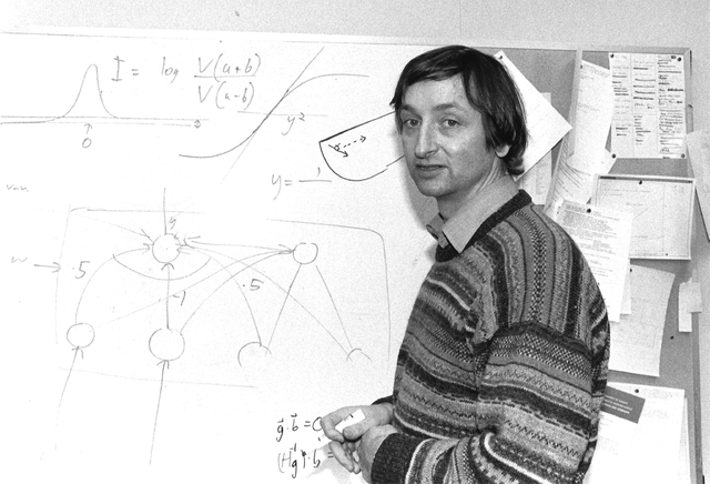
LeCun, Yann, Yoshua Bengio, and Geoffrey Hinton. “Deep Learning.” Nature 521, no. 7553 (May 1, 2015): 436–44. https://doi.org/10.1038/nature14539.
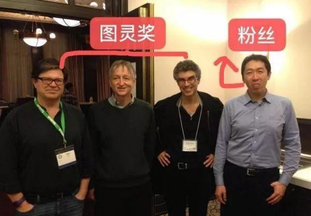
Followers
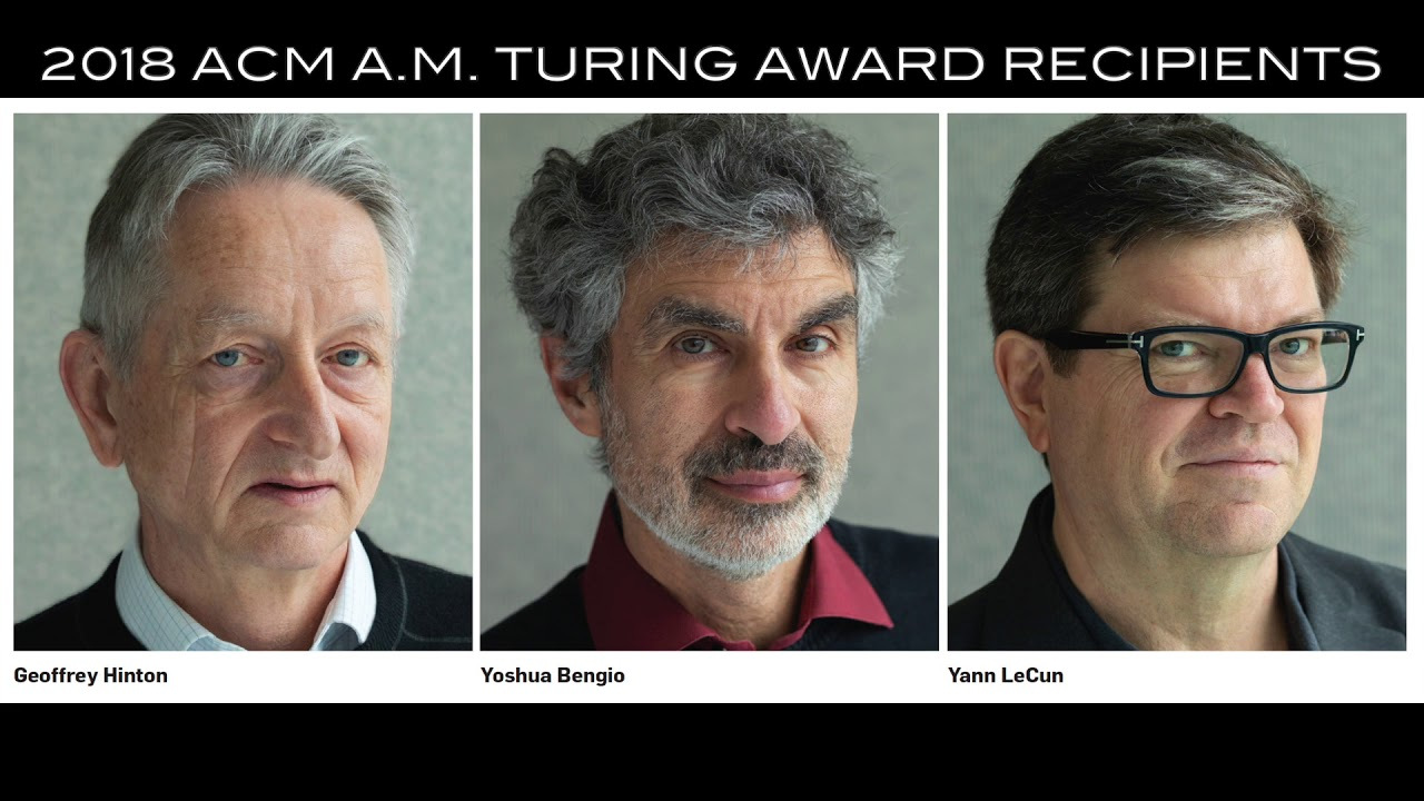
Turing Award
Geoffrey Hinton
Yoshua Bengio
Yann LeCun
Jen-Hsun Huang
Fei-Fei Li
Bill Dally
The Queen Elizabeth Prize for Engineering
(5th Nov, 2025)
quit?
resigned
Nobel Prize in Physics (2024)
LawZero
+
+
=
# GW: DL
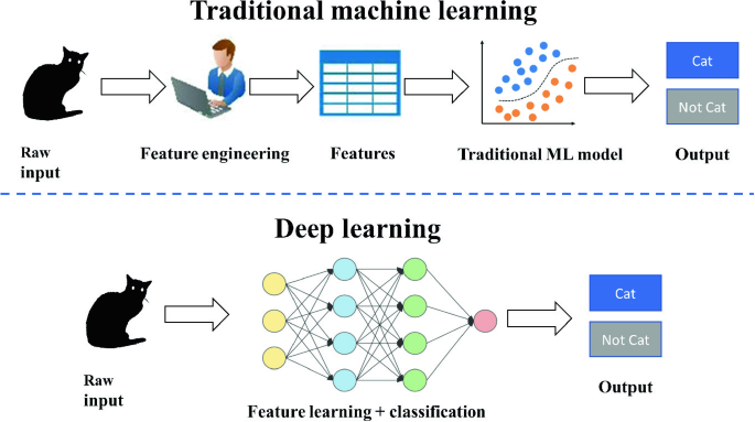
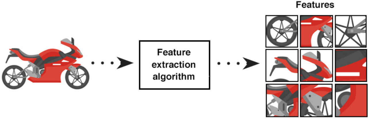
In practice, feature design often matters more than the classifier itself.
Deep Learning: An end-to-end learning paradigm
Enables learning of complex nonlinear mappings.
Shifts from manual knowledge encoding → learning from data
From divide-and-conquer → holistic consideration
From algorithm-focused → data-focused
# GW: DL
# GW: DL
# GW: DL
# GW: DL
Essence: Deep learning uses multi-layer models and large-scale training data (including unlabeled data) to learn more useful features, ultimately improving classification or prediction accuracy.
The deep model is the means; feature learning is the goal.
Differences from Shallow Learning:
Emphasizes model depth, typically with 5–10+ hidden layers;
Highlights feature learning: through layer-by-layer transformations, raw features are mapped into new feature spaces, making classification or prediction easier. Compared to manually designed features, learning from large-scale data better captures the rich intrinsic information of the data.
# GW: DL
# GW: DL
# GW: DL
2003 年,Yann LeCun 等人在 NEC 实验室的使用CNN进行人脸检测。
# GW: DL
在90年代,人工神经网络缺少严格的数学理论支撑,统计学习大发展。 Vapnik提出支持向量机(SVM),改进了感知器的一些缺陷(例如创建灵活的特征而不是手编的非适应的特征)。它同样解决了线性不可分问题,但是对比神经网络有全方位优势:
SVM (support vector machines)
# GW: DL
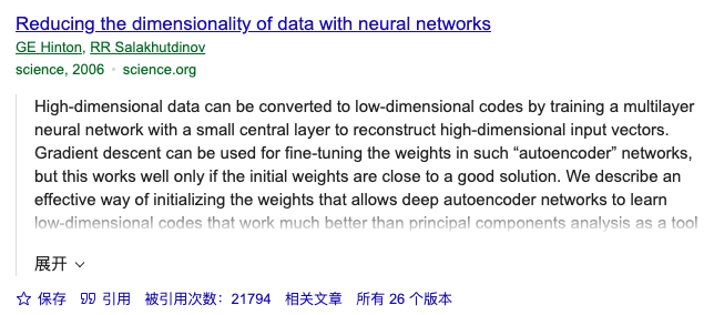
被 Hinton 首次定义为深度学习过程
# GW: DL
# GW: DL
# GW: DL
# GW: DL
Who Am I
— A quick intro and how I got into this field
What Is Machine Learning?
— The basics and why it matters
Deep Learning: When Machines Start to See and Think
— From neural networks to powerful representations
Gravitational Waves Meet Machine Learning
— How ML is reshaping data analysis in GW astronomy
Let’s Get Practical: Searching for Gravitational Waves
— A hands-on look at applying ML in real GW searches
LLMs for Gravitational Waves: My Ongoing Work
— Towards automated and interpretable scientific discovery
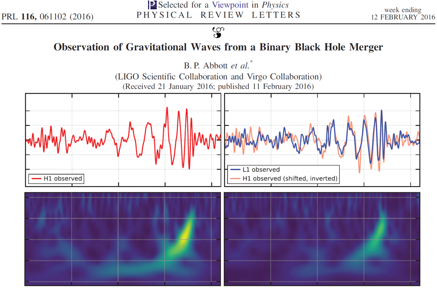
# GW
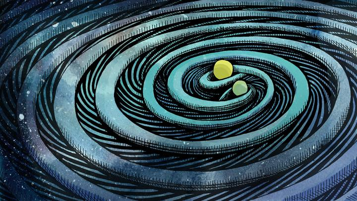
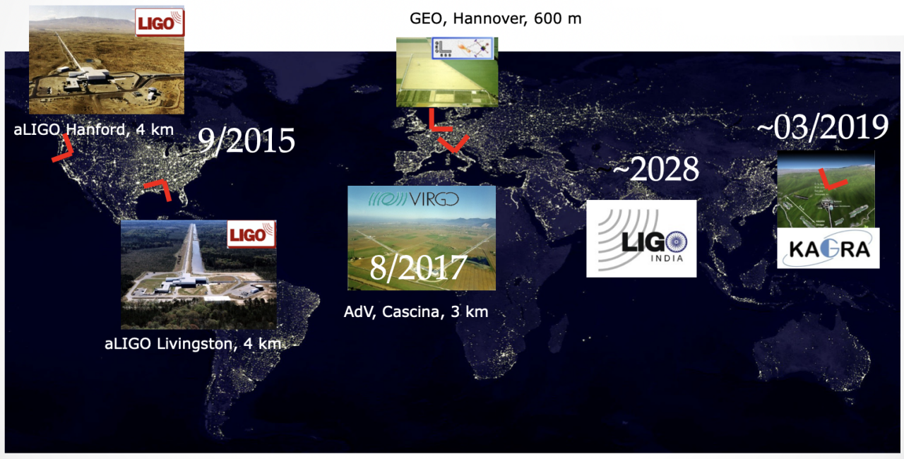
Gravitational waves (GW) are a strong field effect in General Relativity, ripples in the fabric of spacetime caused by accelerating massive objects.
Compact Binary Coalescences
LIGO-Virgo-KAGRA-...
—— Bernard F. Schutz
DOI: 10.1063/1.1629411
# GW
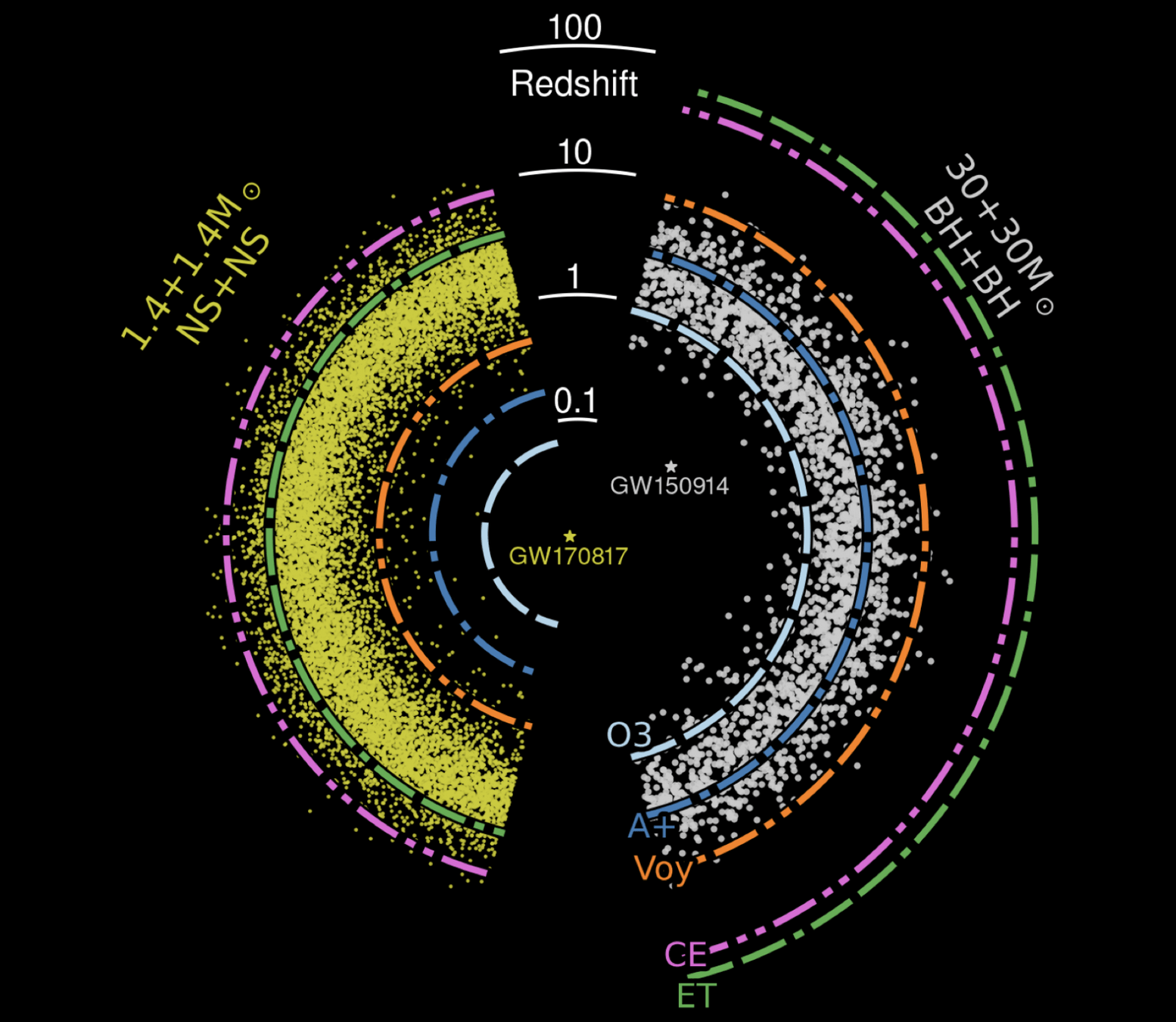
GW Data Characteristics
LIGO-VIRGO-KAGRA
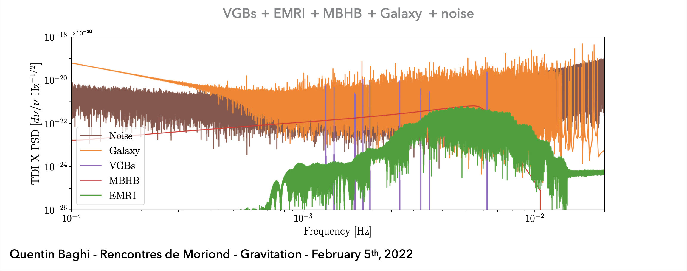
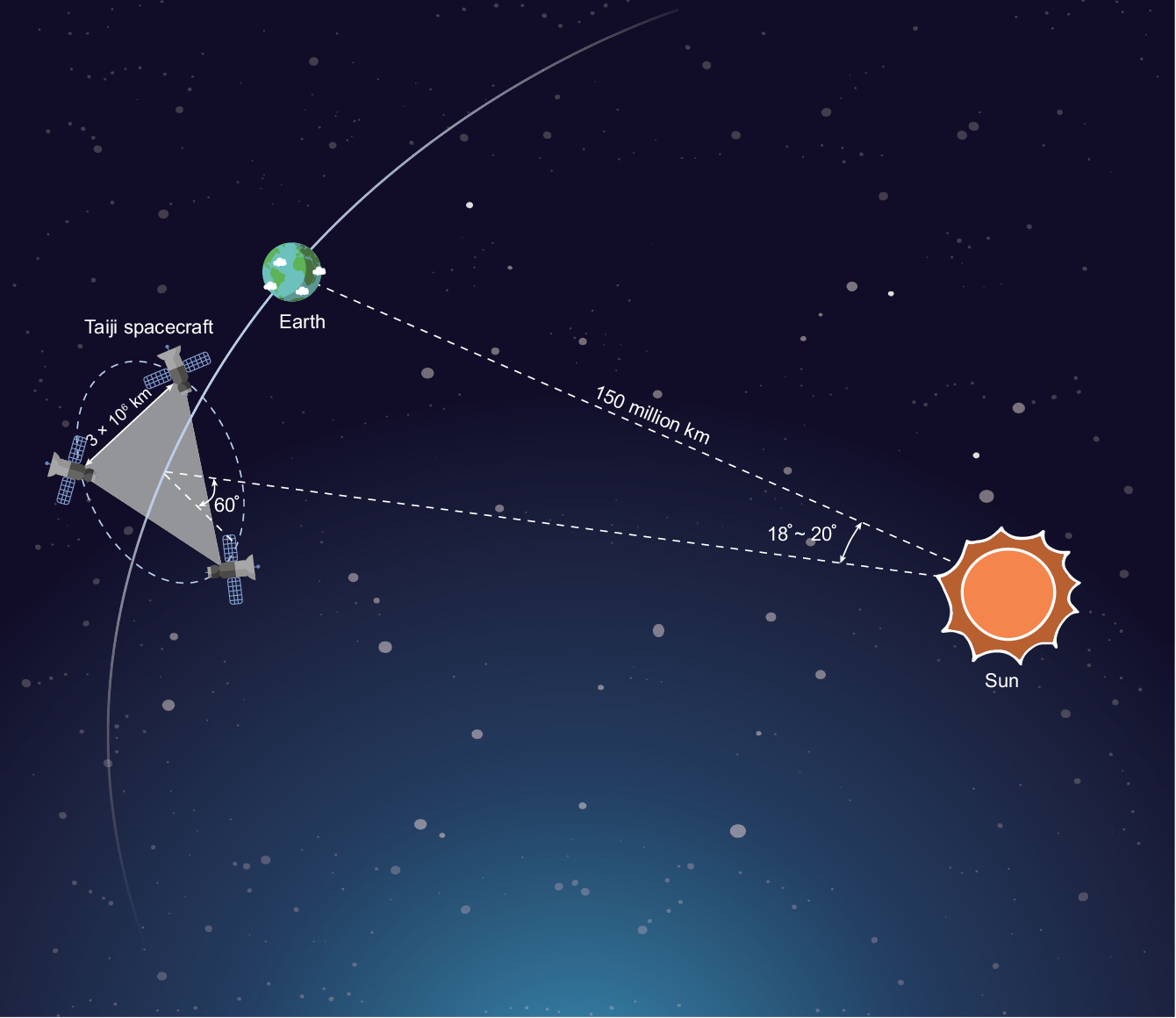
LISA Project
Noise: non-Gaussian and non-stationary
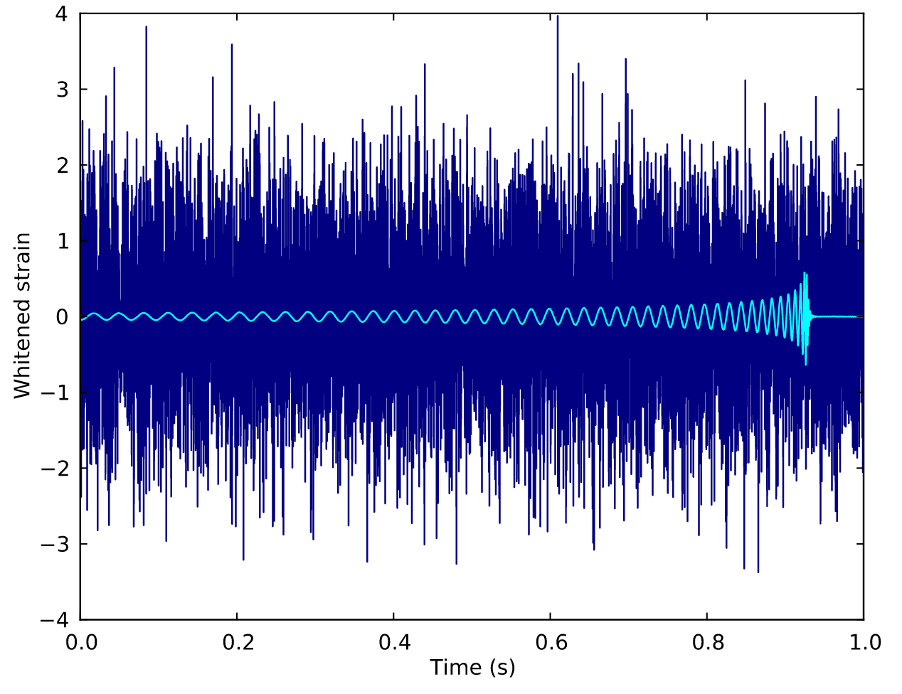
Signal challenges:
(Earth-based) A low signal-to-noise ratio (SNR) which is typically about 1/100 of the noise amplitude (-60 dB).
(Space-based) A superposition of all GW signals (e.g.: 104 of GBs, 10~102 of SMBHs, and 10~103 of EMRIs, etc.) received during the mission's observational run.
Matched Filtering Techniques (匹配滤波方法)
In Gaussian and stationary noise environments, the optimal linear algorithm for extracting weak signals
Statistical Approaches
Frequentist Testing:
Bayesian Testing:
# GW
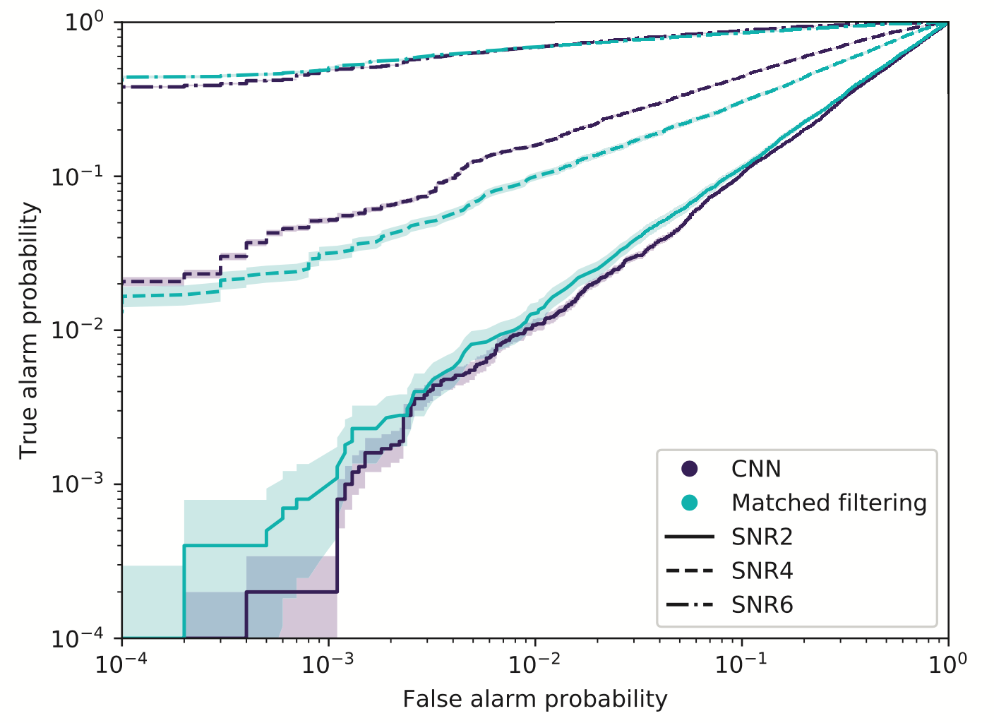
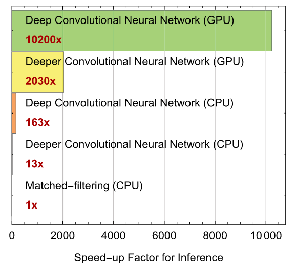
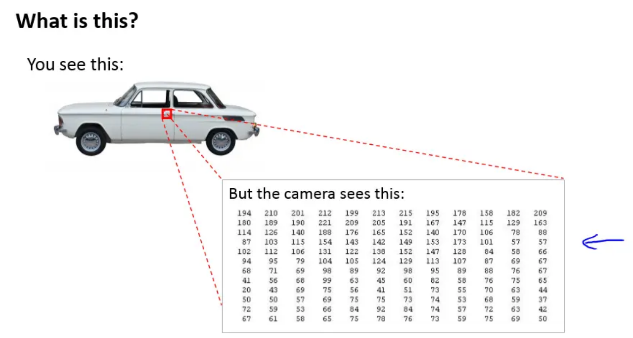
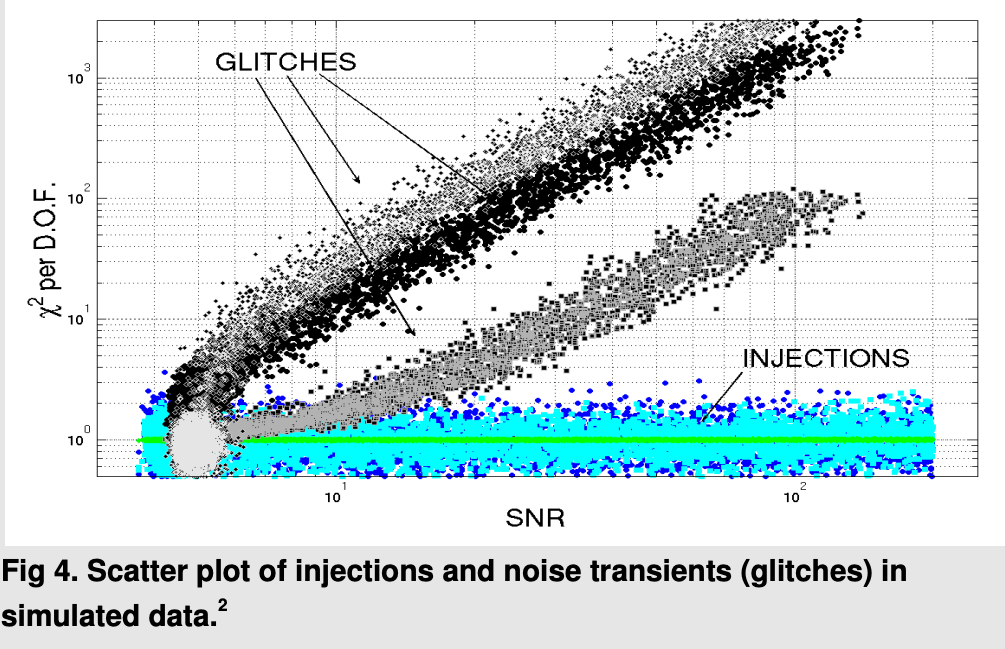
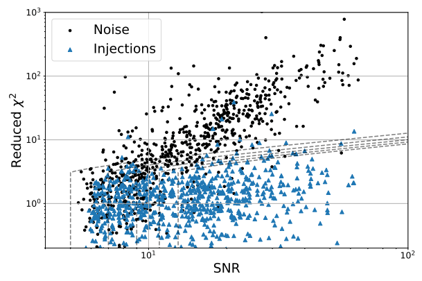
Core Insight from Computer Vision
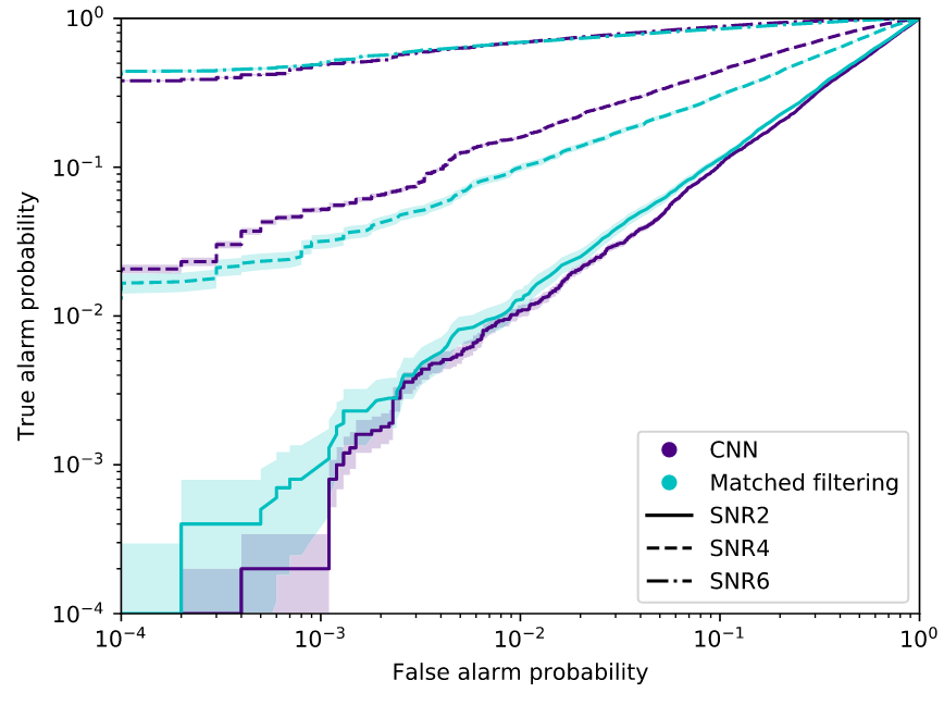
Performance Analysis
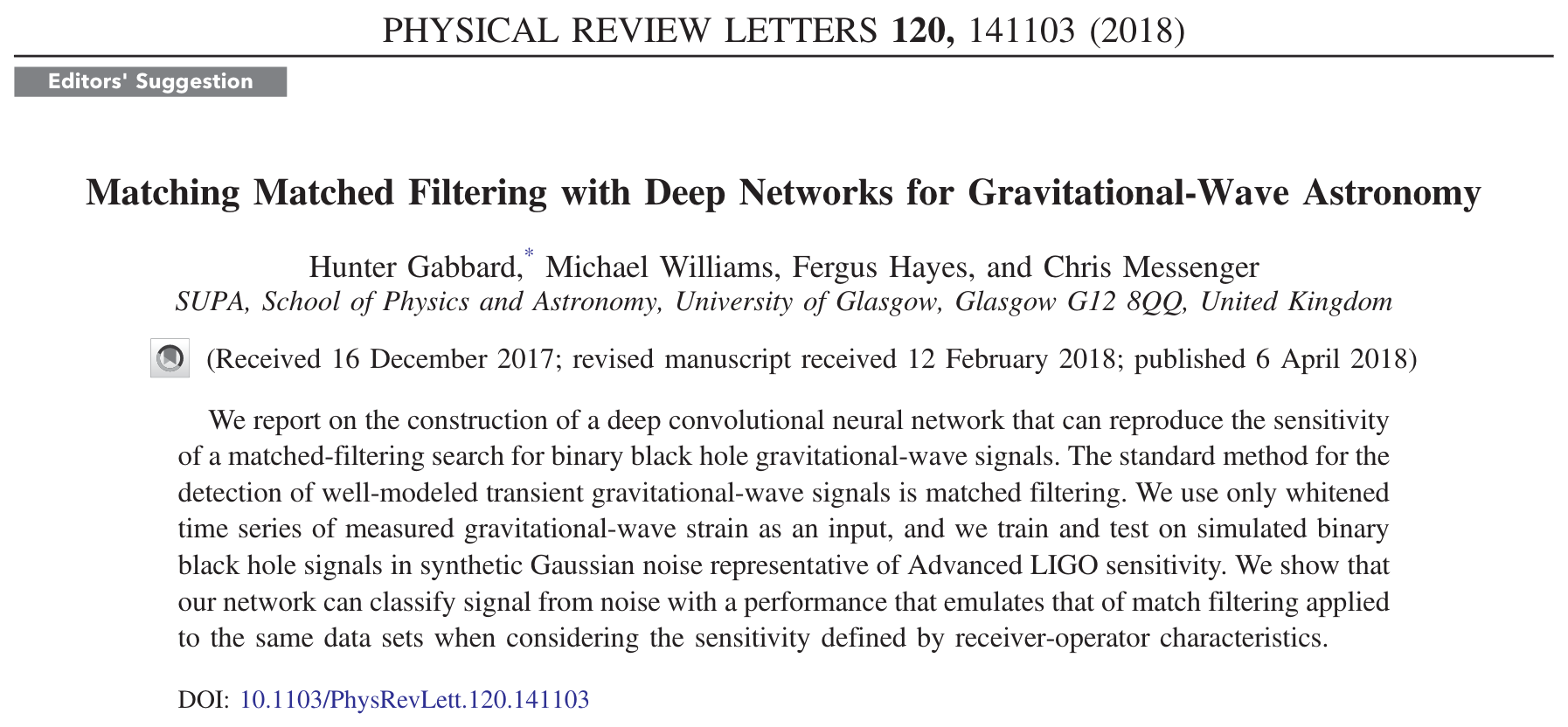
Pioneering Research Publications
PRL, 2018, 120(14): 141103.
PRD, 2018, 97(4): 044039.
# GW
A hands-on look at applying ML in real GW searches:
https://github.com/iphysresearch/GWData-Bootcamp
=> 2023/deep_learning/baseline/baseline_2025FQCP.ipynb
# GW
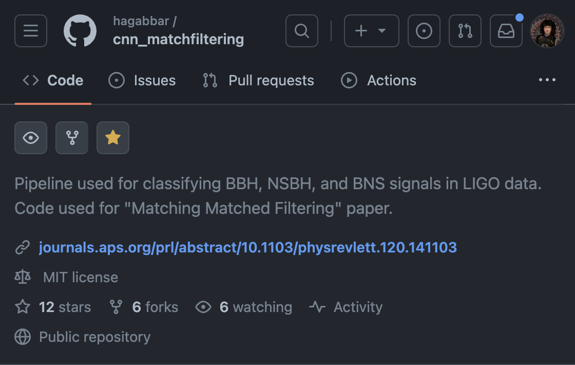
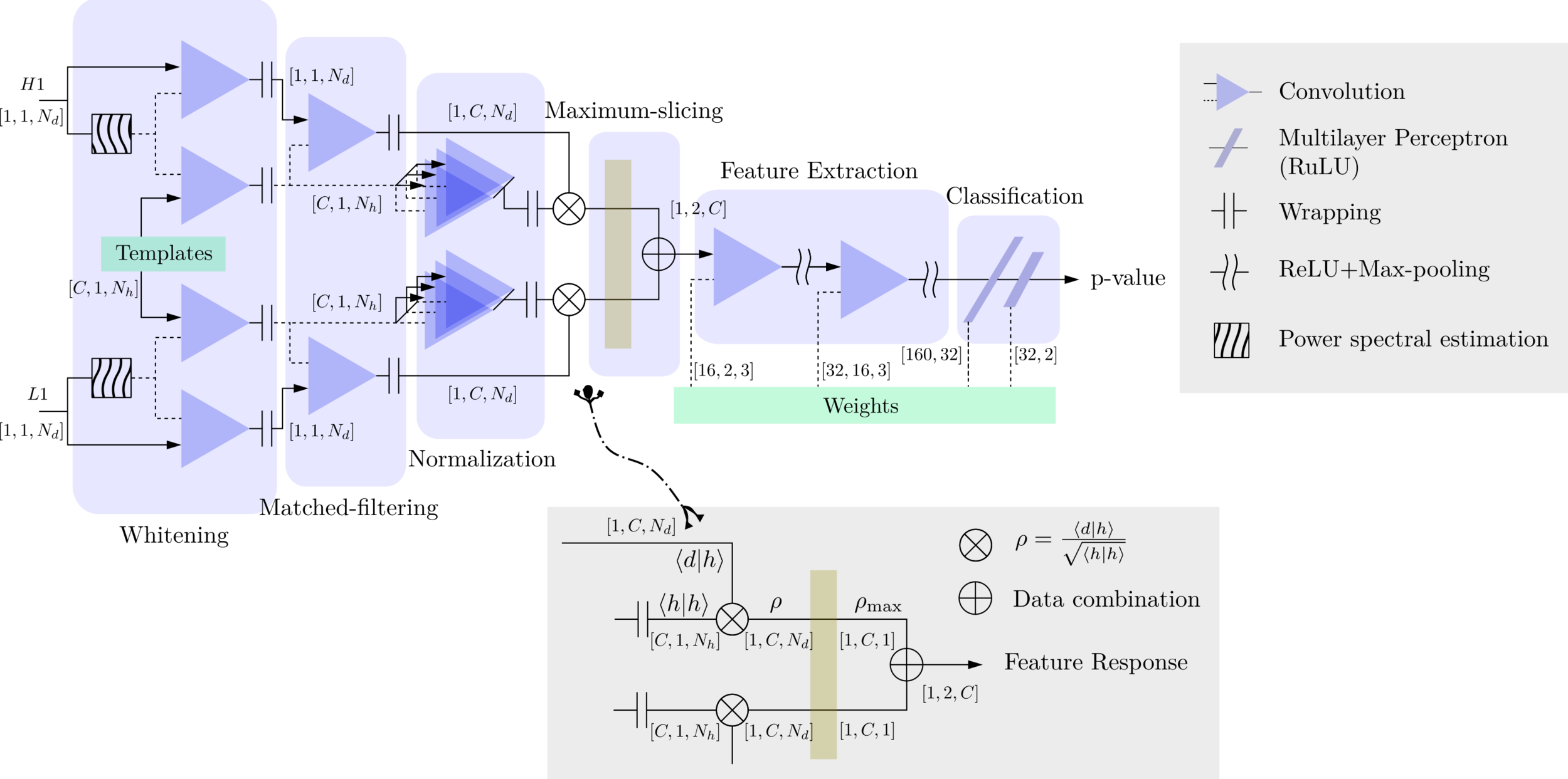
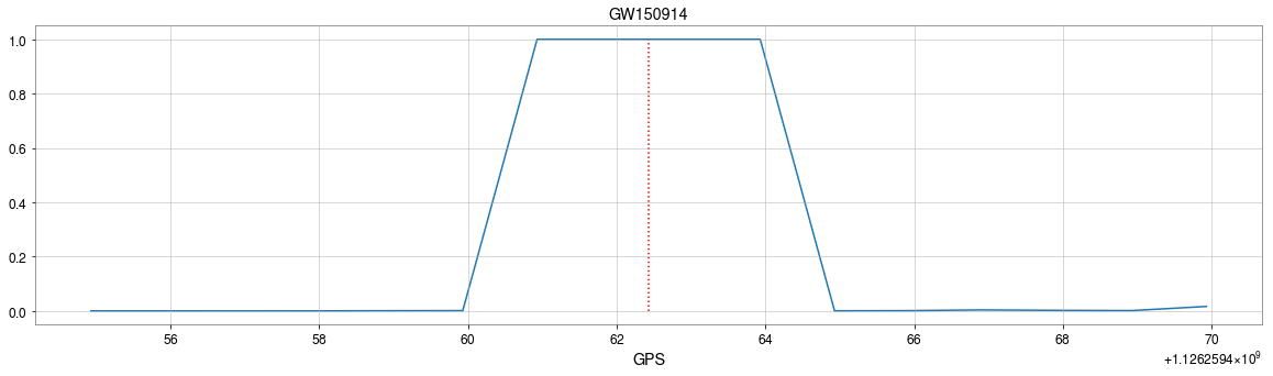
Matched-filtering Convolutional Neural Network (MFCNN)
HW, SC Wu, ZJ CAO, et al. PRD 101, 10 (2020): 104003
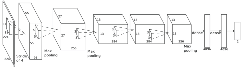
Convolutional Neural Network (ConvNet or CNN)
feature extraction
classifier
>> Is it matched-filtering ?
>> Wait, It can be matched-filtering!
GW150914
GW150914
# GW
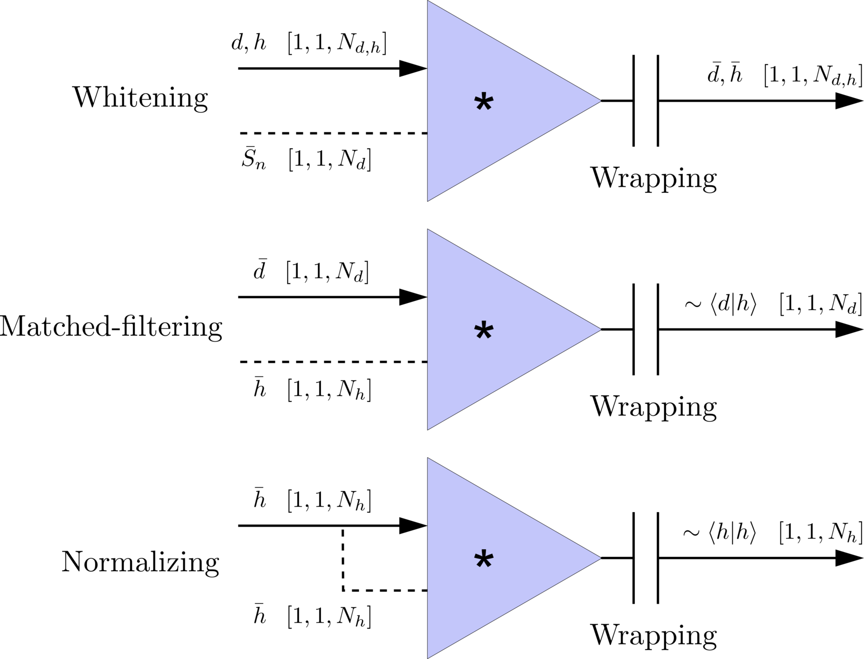
Transform matched-filtering method from frequency domain to time domain.
The square of matched-filtering SNR for a given data \(d(t) = n(t)+h(t)\):
\(S_n(|f|)\) is the one-sided average PSD of \(d(t)\)
where
Deep Learning Framework
Time Domain
(matched-filtering)
(normalizing)
(whitening)
Frequency Domain
# GW
Transform matched-filtering method from frequency domain to time domain.
The square of matched-filtering SNR for a given data \(d(t) = n(t)+h(t)\):
\(S_n(|f|)\) is the one-sided average PSD of \(d(t)\)
where
Deep Learning Framework
Time Domain
(matched-filtering)
(normalizing)
(whitening)
Frequency Domain
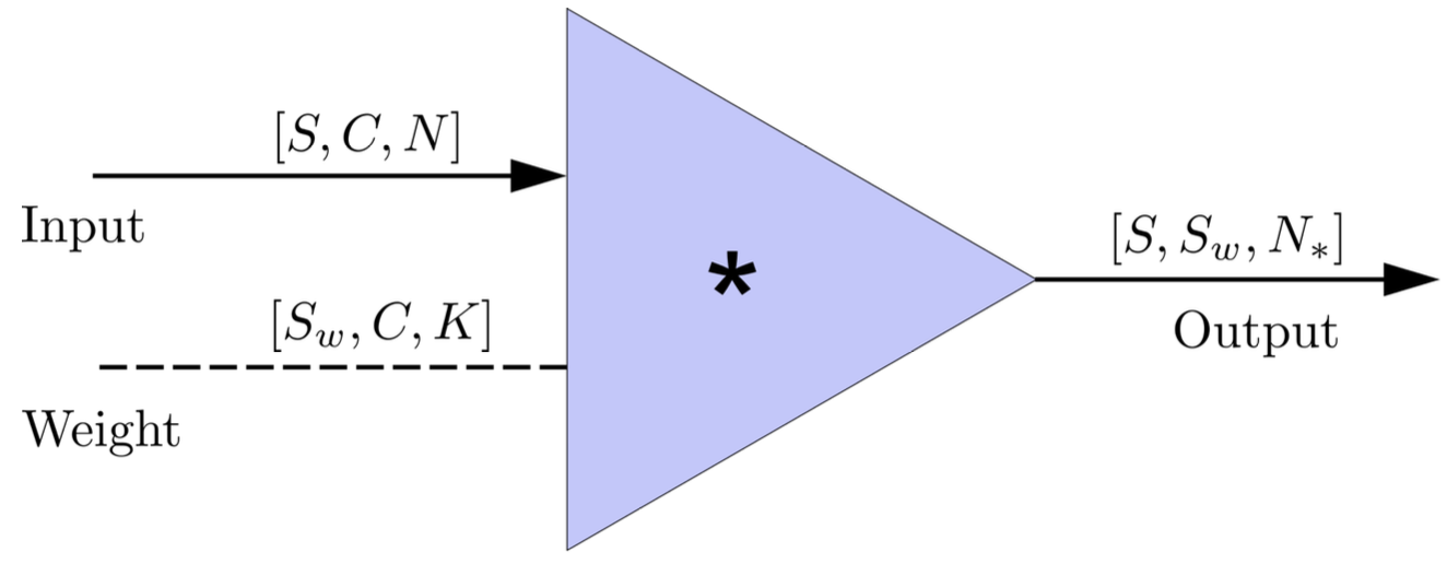
FYI: \(N_\ast = \lfloor(N-K+2P)/S\rfloor+1\)
(A schematic illustration for a unit of convolution layer)
# GW
import mxnet as mx
from mxnet import nd, gluon
from loguru import logger

def MFCNN(fs, T, C, ctx, template_block, margin, learning_rate=0.003):
    logger.success('Loading MFCNN network!')
    net = gluon.nn.Sequential()
    with net.name_scope():
        net.add(MatchedFilteringLayer(mod=fs*T, fs=fs,
                                      template_H1=template_block[:,:1],
                                      template_L1=template_block[:,-1:]))
        net.add(CutHybridLayer(margin = margin))
        net.add(Conv2D(channels=16, kernel_size=(1, 3), activation='relu'))
        net.add(MaxPool2D(pool_size=(1, 4), strides=2))
        net.add(Conv2D(channels=32, kernel_size=(1, 3), activation='relu'))
        net.add(MaxPool2D(pool_size=(1, 4), strides=2))
        net.add(Flatten())
        net.add(Dense(32))
        net.add(Activation('relu'))
        net.add(Dense(2))
	# Initialize parameters of all layers
    net.initialize(mx.init.Xavier(magnitude=2.24), ctx=ctx, force_reinit=True)
    return net
1 sec duration
35 templates used
Explainable AI Approach
Matched-filtering Convolutional Neural Network (MFCNN)
The available codes (2019): https://gist.github.com/iphysresearch/a00009c1eede565090dbd29b18ae982c
HW, SC Wu, ZJ CAO, et al. PRD 101, 10 (2020): 104003
# GW
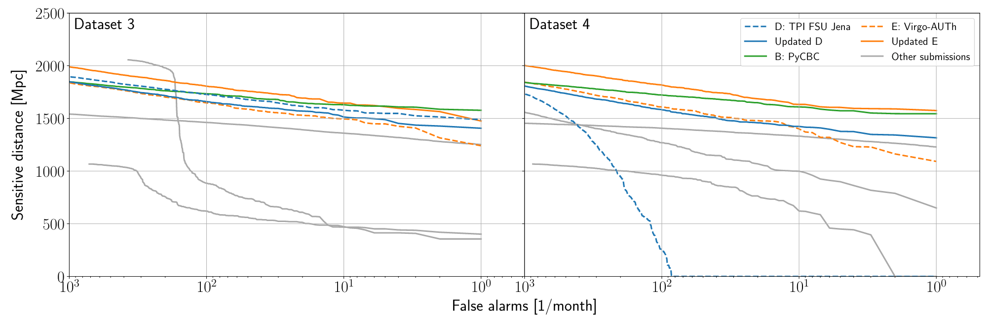
Benchmark Results
Publications
Key Findings
Note on Benchmark Limitations:
Outperforming PyCBC doesn't conclusively prove that matched filtering is inferior to AI methods. This is both because the dataset represents a specific distribution and because PyCBC settings could be further optimized for this particular benchmark.
arXiv:2501.13846 [gr-qc]
Phys. Rev. D 107, 023021 (2023)
# GW
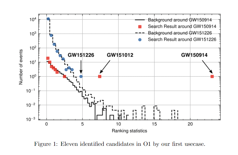
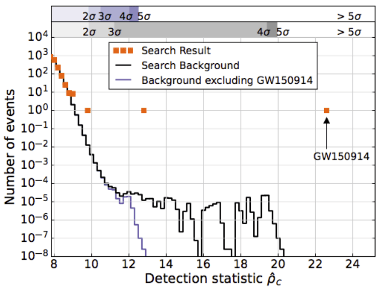
AI Model Denoising
Our Model's Detection Statistics
LVK Official Detection Statistics
Signal denoising visualization using our deep learning model (Transformer-based)
Detection statistics from our AI model showing O1 events
HW et al 2024 MLST 5 015046
GW151226
GW151012
Official detection statistics from LVK collaboration
LVK. PRD (2016). arXiv:1602.03839
# GW
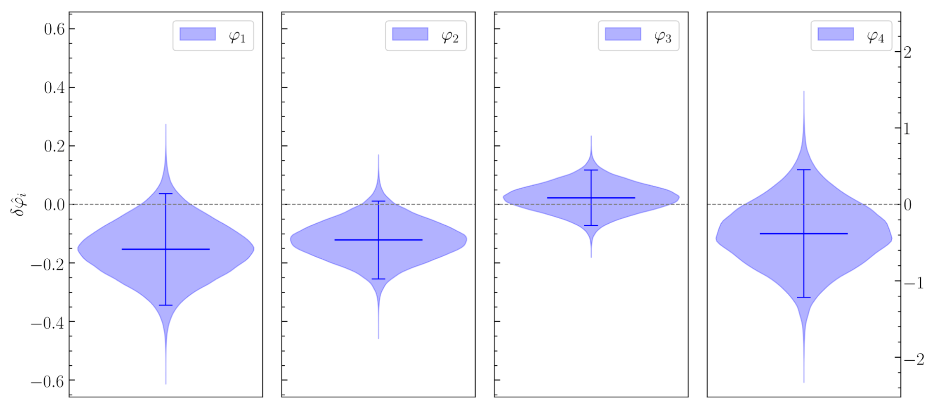
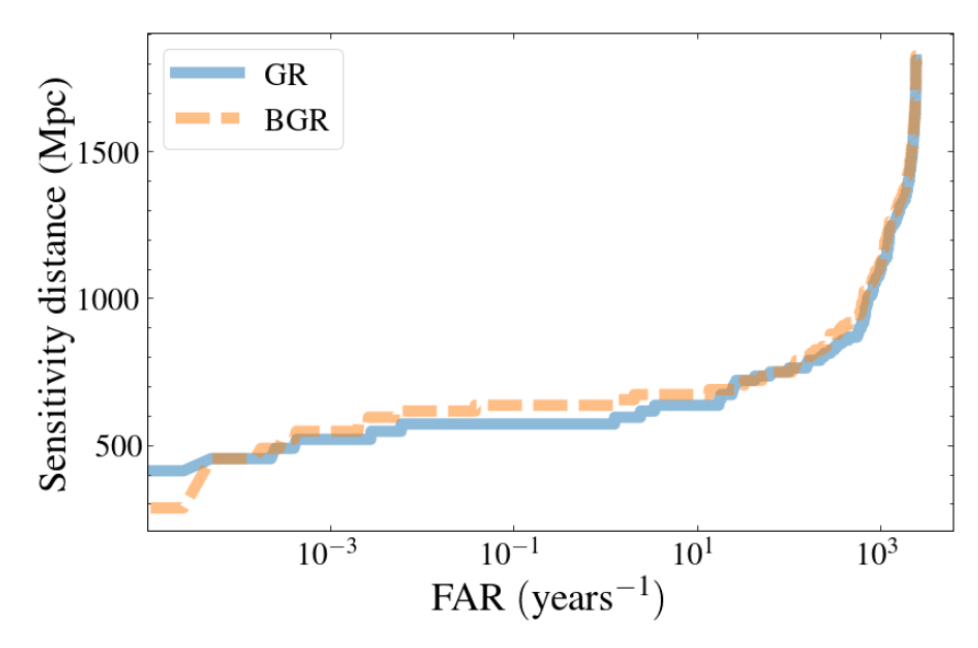
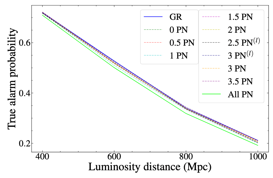
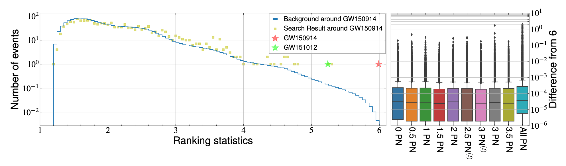
B. P. Abbott et al. (LIGO-Virgo), PRD 100, 104036 (2019).
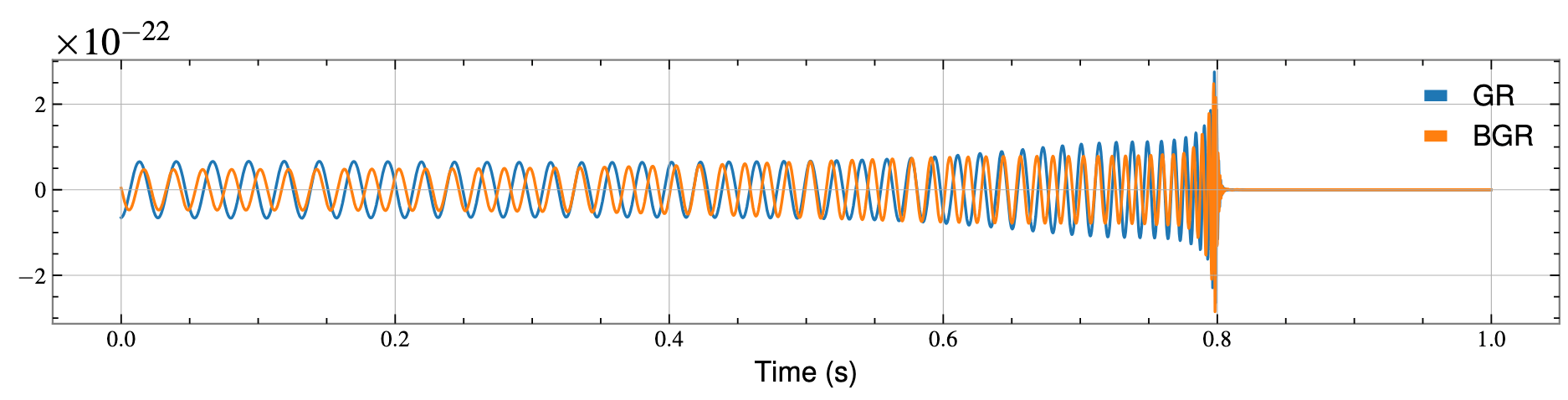
Yu-Xin Wang, Xiaotong Wei, Chun-Yue Li, Tian-Yang Sun, Shang-Jie Jin, He Wang*, Jing-Lei Cui, Jing-Fei Zhang, and Xin Zhang*. “Search for Exotic Gravitational Wave Signals beyond General Relativity Using Deep Learning.” PRD 112 (2), 024030. e-Print: arXiv:2410.20129 [grqc]
# GW
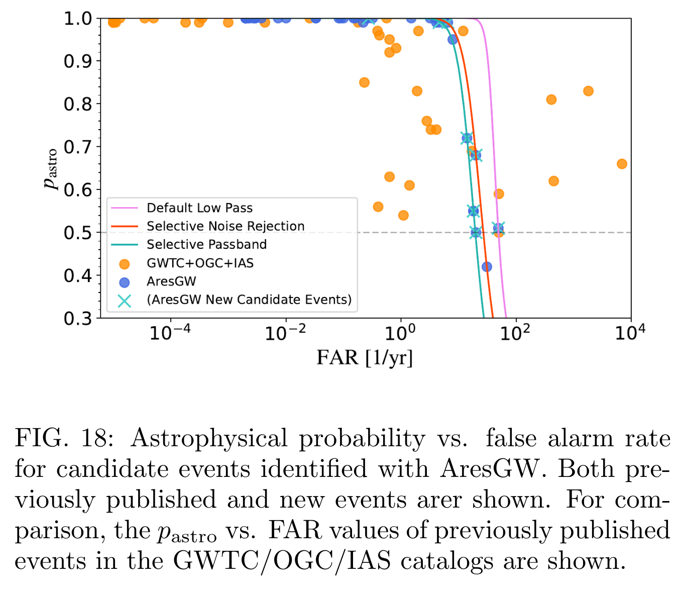
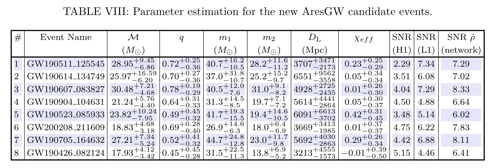
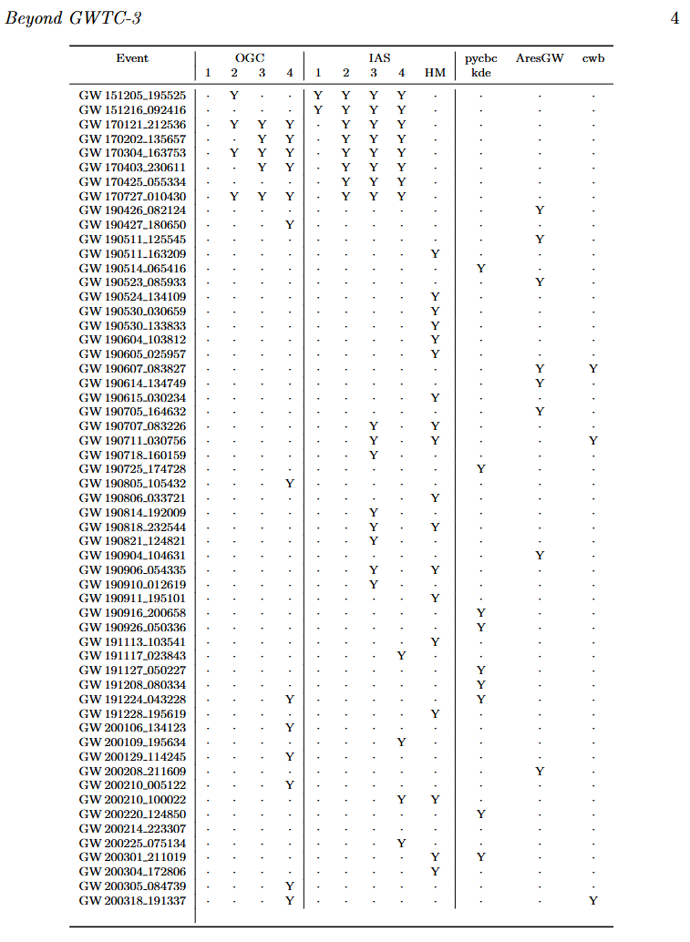
arXiv:2407.07820 [gr-qc]
Recent AI Discoveries & Validation Hurdles:
Search
PE
Rate
Key Insight:
# GW
Recent AI Discoveries & Validation Hurdles:
Search
PE
Rate
Key Insight:
Credit: DCC-XXXXXXXX
# GW
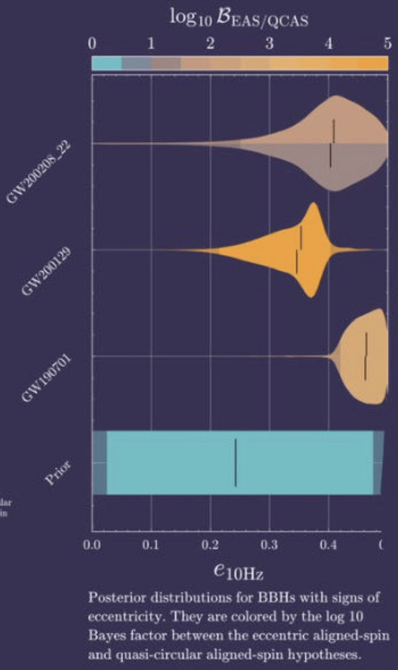
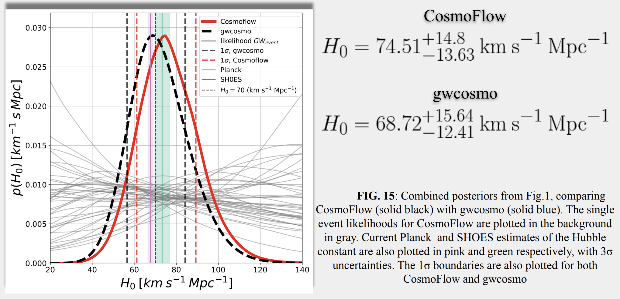
Parameter Estimation Challenges with AI Models:
arXiv:2404.14286
Phys. Rev. D 109, 123547 (2024)
hewang@ucas.ac.cn
See more:
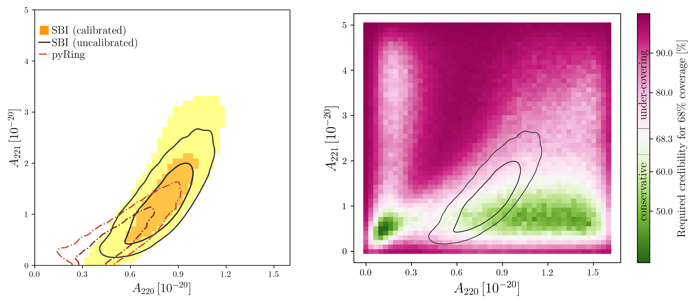
PRD 108, 4 (2023): 044029.
Neural Posterior Estimation with Guaranteed Exact Coverage: The Ringdown of GW150914
# GW
Sci4MLGW@ICERM (June 2025)
Parameter Estimation Challenges with AI Models:
arXiv:2404.14286
Phys. Rev. D 109, 123547 (2024)
See more:
PRD 108, 4 (2023): 044029.
Neural Posterior Estimation with Guaranteed Exact Coverage: The Ringdown of GW150914
Who Am I
— A quick intro and how I got into this field
What Is Machine Learning?
— The basics and why it matters
Deep Learning: When Machines Start to See and Think
— From neural networks to powerful representations
Gravitational Waves Meet Machine Learning
— How ML is reshaping data analysis in GW astronomy
Let’s Get Practical: Searching for Gravitational Waves
— A hands-on look at applying ML in real GW searches
LLMs for Gravitational Waves: My Ongoing Work
— Towards automated and interpretable scientific discovery
Motivation 1: Traditional methods heavily rely on manually designed filters and statistics.
Motivation 2: AI interpretability challenge: Discoveries vs. Validation.
hewang@ucas.ac.cn
Motivation I: Linear template method using prior data
Motivation II: Black-box data-driven learning methods
The strict requirements for algorithm discovery
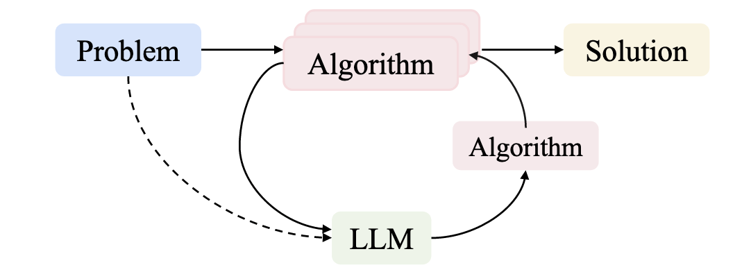
Large Language Models (LLMs) as Designers
external_knowledge
(constraint)
Fitness
import numpy as np
import scipy.signal as signal
def pipeline_v1(strain_h1: np.ndarray, strain_l1: np.ndarray, times: np.ndarray) -> tuple[np.ndarray, np.ndarray, np.ndarray]:
def data_conditioning(strain_h1: np.ndarray, strain_l1: np.ndarray, times: np.ndarray) -> tuple[np.ndarray, np.ndarray, np.ndarray]:
window_length = 4096
dt = times[1] - times[0]
fs = 1.0 / dt
def whiten_strain(strain):
strain_zeromean = strain - np.mean(strain)
freqs, psd = signal.welch(strain_zeromean, fs=fs, nperseg=window_length,
window='hann', noverlap=window_length//2)
smoothed_psd = np.convolve(psd, np.ones(32) / 32, mode='same')
smoothed_psd = np.maximum(smoothed_psd, np.finfo(float).tiny)
white_fft = np.fft.rfft(strain_zeromean) / np.sqrt(np.interp(np.fft.rfftfreq(len(strain_zeromean), d=dt), freqs, smoothed_psd))
return np.fft.irfft(white_fft)
whitened_h1 = whiten_strain(strain_h1)
whitened_l1 = whiten_strain(strain_l1)
return whitened_h1, whitened_l1, times
def compute_metric_series(h1_data: np.ndarray, l1_data: np.ndarray, time_series: np.ndarray) -> tuple[np.ndarray, np.ndarray]:
fs = 1 / (time_series[1] - time_series[0])
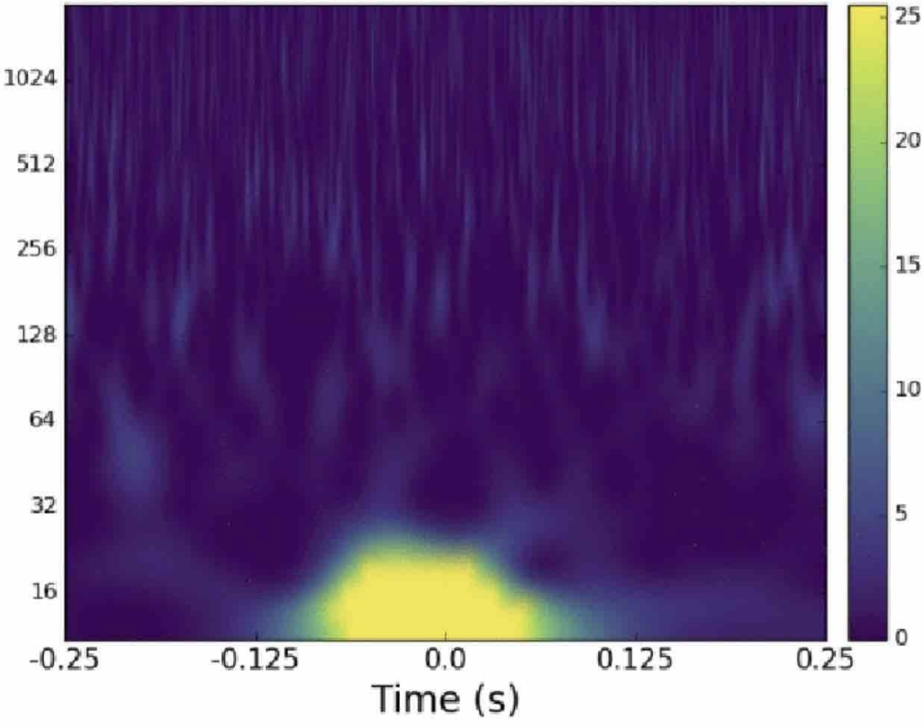
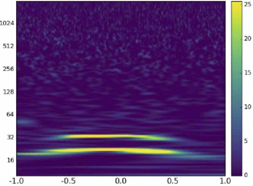
f_h1, t_h1, Sxx_h1 = signal.spectrogram(h1_data, fs=fs, nperseg=256, noverlap=128, mode='magnitude', detrend=False)
f_l1, t_l1, Sxx_l1 = signal.spectrogram(l1_data, fs=fs, nperseg=256, noverlap=128, mode='magnitude', detrend=False)
tf_metric = np.mean((Sxx_h1**2 + Sxx_l1**2) / 2, axis=0)
gps_mid_time = time_series[0] + (time_series[-1] - time_series[0]) / 2
metric_times = gps_mid_time + (t_h1 - t_h1[-1] / 2)
return tf_metric, metric_times
def calculate_statistics(tf_metric, t_h1):
background_level = np.median(tf_metric)
peaks, _ = signal.find_peaks(tf_metric, height=background_level * 1.0, distance=2, prominence=background_level * 0.3)
peak_times = t_h1[peaks]
peak_heights = tf_metric[peaks]
peak_deltat = np.full(len(peak_times), 10.0) # Fixed uncertainty value
return peak_times, peak_heights, peak_deltat
whitened_h1, whitened_l1, data_times = data_conditioning(strain_h1, strain_l1, times)
tf_metric, metric_times = compute_metric_series(whitened_h1, whitened_l1, data_times)
peak_times, peak_heights, peak_deltat = calculate_statistics(tf_metric, metric_times)
return peak_times, peak_heights, peak_deltat
Input: H1 and L1 detector strains, time array | Output: Event times, significance values, and time uncertainties
external_knowledge
(constraint)
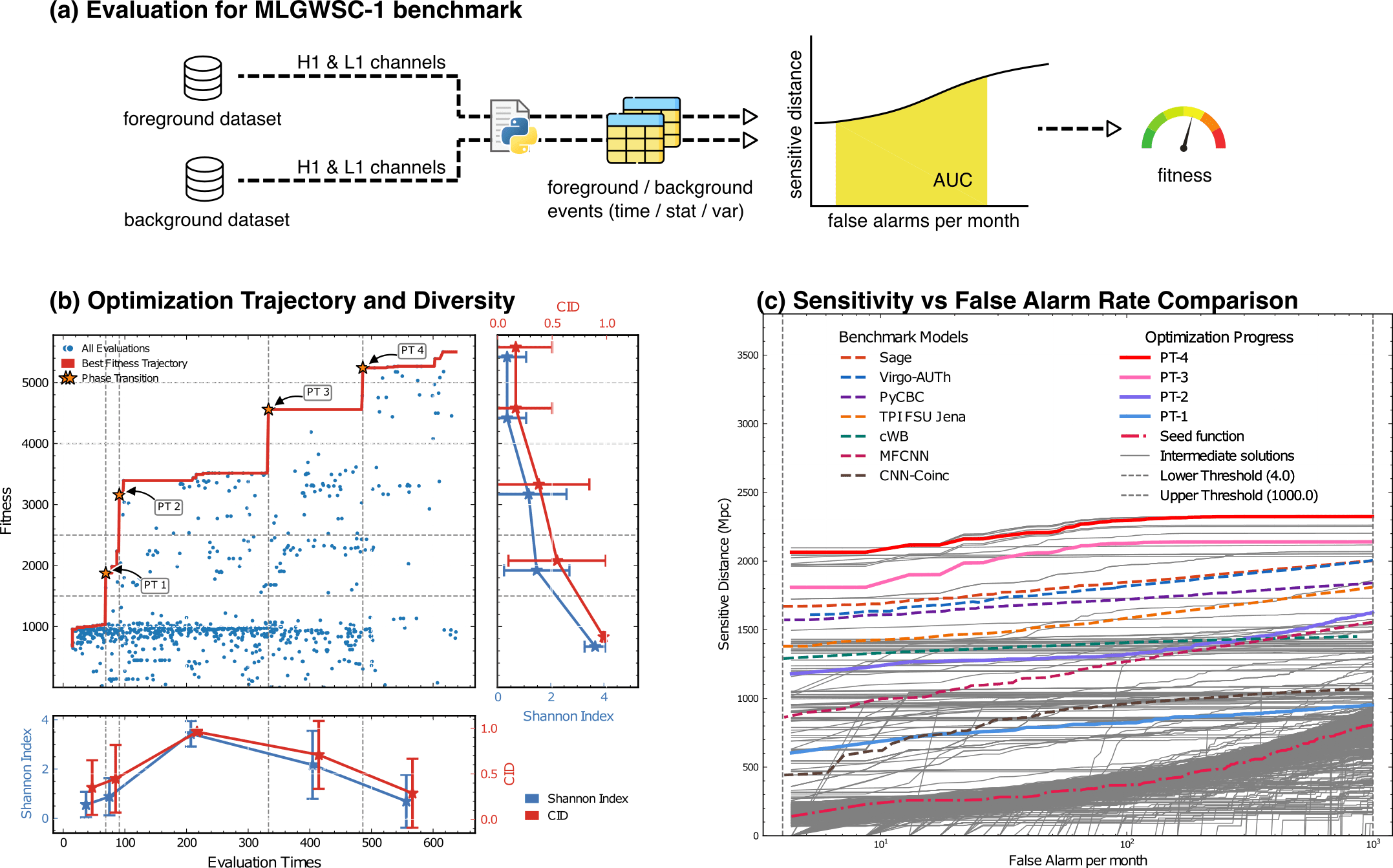
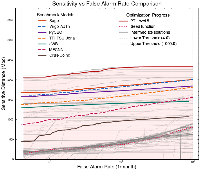
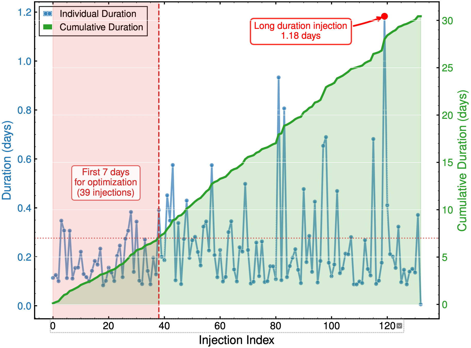
Optimization Target: Maximizing Area Under Curve (AUC) in the 1-1000Hz false alarms per-year range, balancing detection sensitivity and false alarm rates across algorithm generations
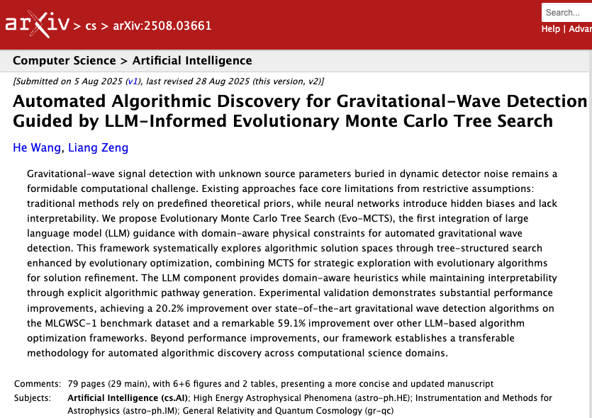
HW & ZL, arXiv:2508.03661
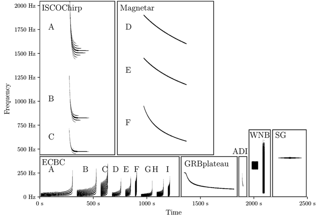
MLGWSC-1 benchmark
Problem: Pipeline Workflow
external_knowledge
(constraint)
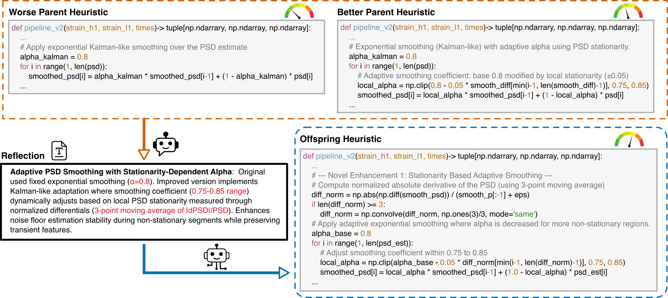
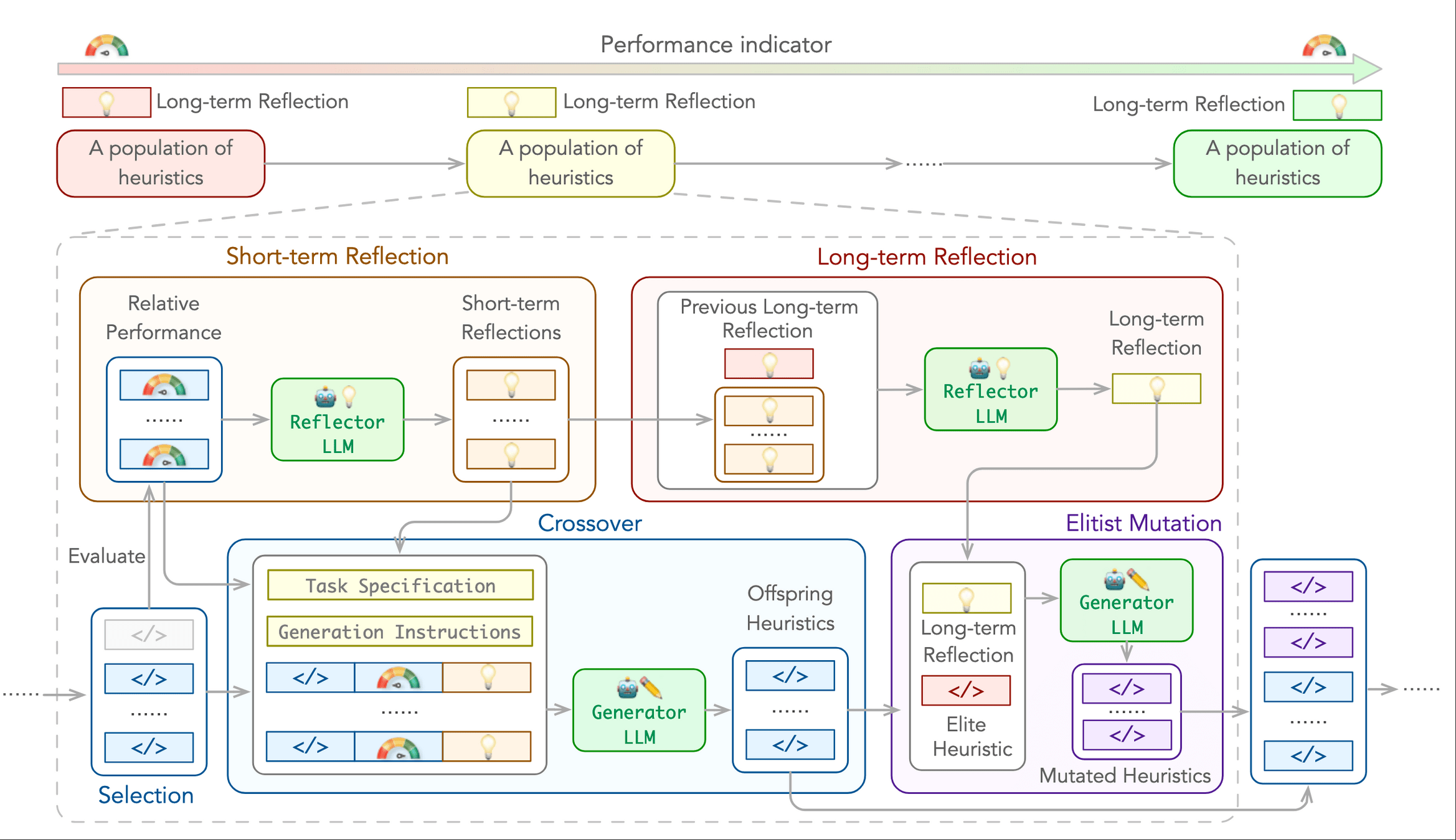
Prompt Structure for Algorithm Evolution
This template guides the LLM to generate optimized gravitational wave detection algorithms by learning from comparative examples.
Key Components:
You are an expert in gravitational wave signal detection algorithms. Your task is to design heuristics that can effectively solve optimization problems.

{prompt_task}

I have analyzed two algorithms and provided a reflection on their differences.

[Worse code]
{worse_code}

[Better code]
{better_code}

[Reflection]
{reflection}

{external_knowledge}

Based on this reflection, please write an improved algorithm according to the reflection.
First, describe the design idea and main steps of your algorithm in one sentence. The description must be inside a brace outside the code implementation. Next, implement it in Python as a function named '{func_name}'.
This function should accept {input_count} input(s): {joined_inputs}. The function should return {output_count} output(s): {joined_outputs}.
{inout_inf} {other_inf}

Do not give additional explanations.
One Prompt Template for MLGWSC1 Algorithm Synthesis
HW & ZL, arXiv:2508.03661
hewang@ucas.ac.cn
Evaluation for MLGWSC-1 benchmark
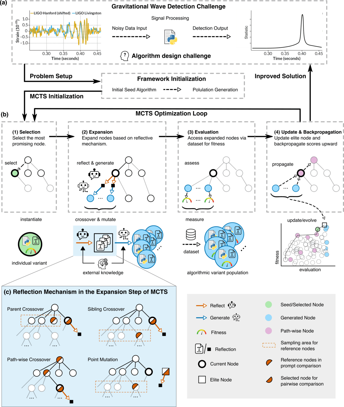
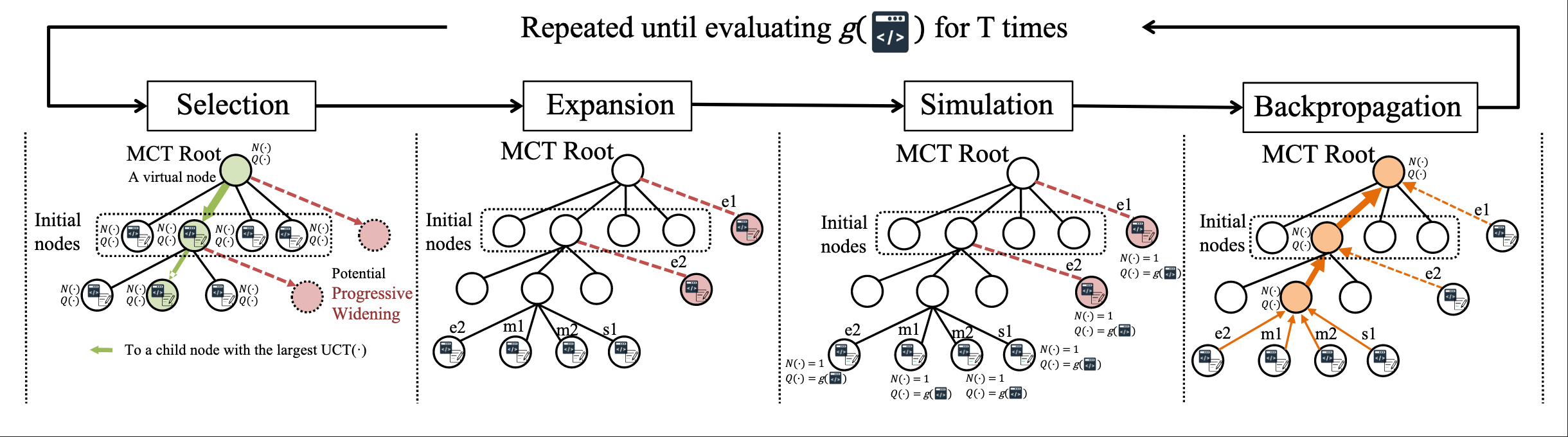
LLM-Driven Algorithmic Evolution Through Reflective Code Synthesis.
LLM-Informed Evo-MCTS for AAD
HW & ZL, arXiv:2508.03661
hewang@ucas.ac.cn
HW & ZL, arXiv:2508.03661
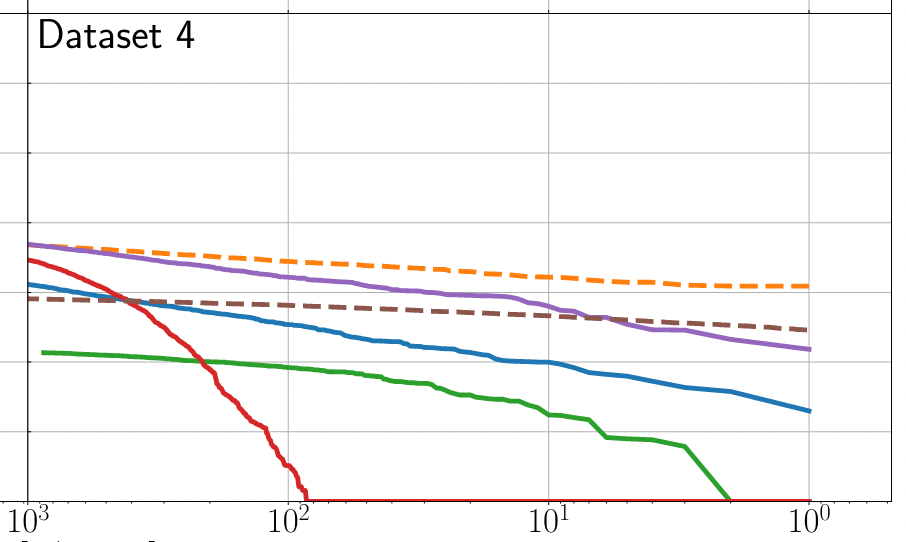
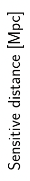
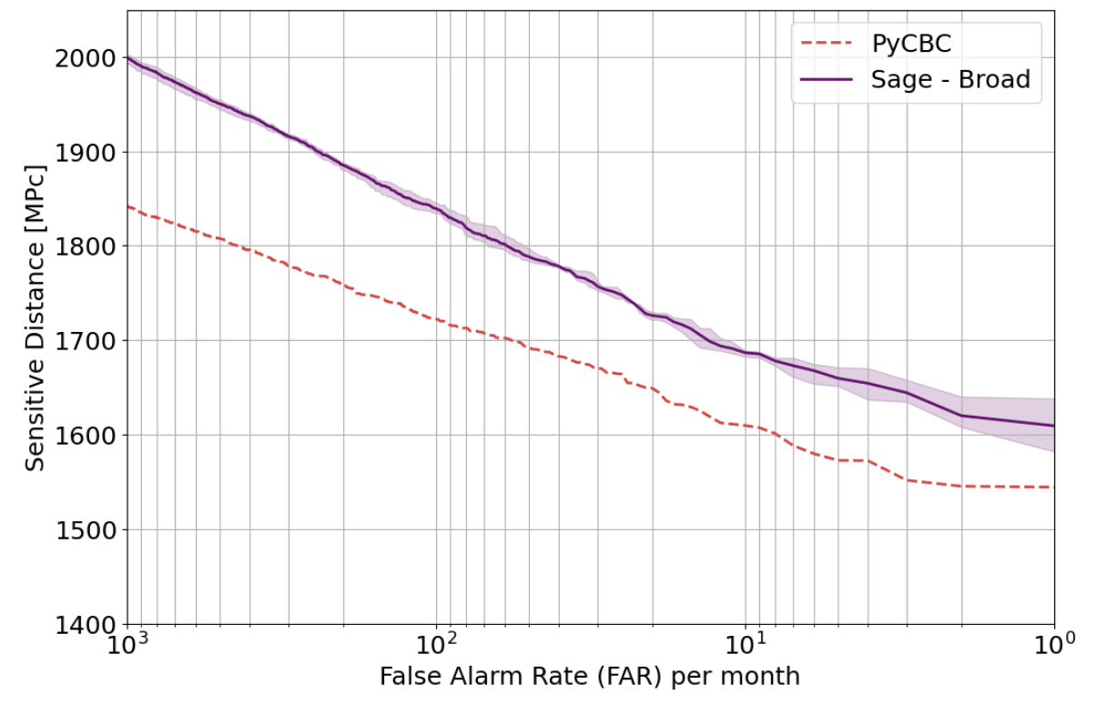
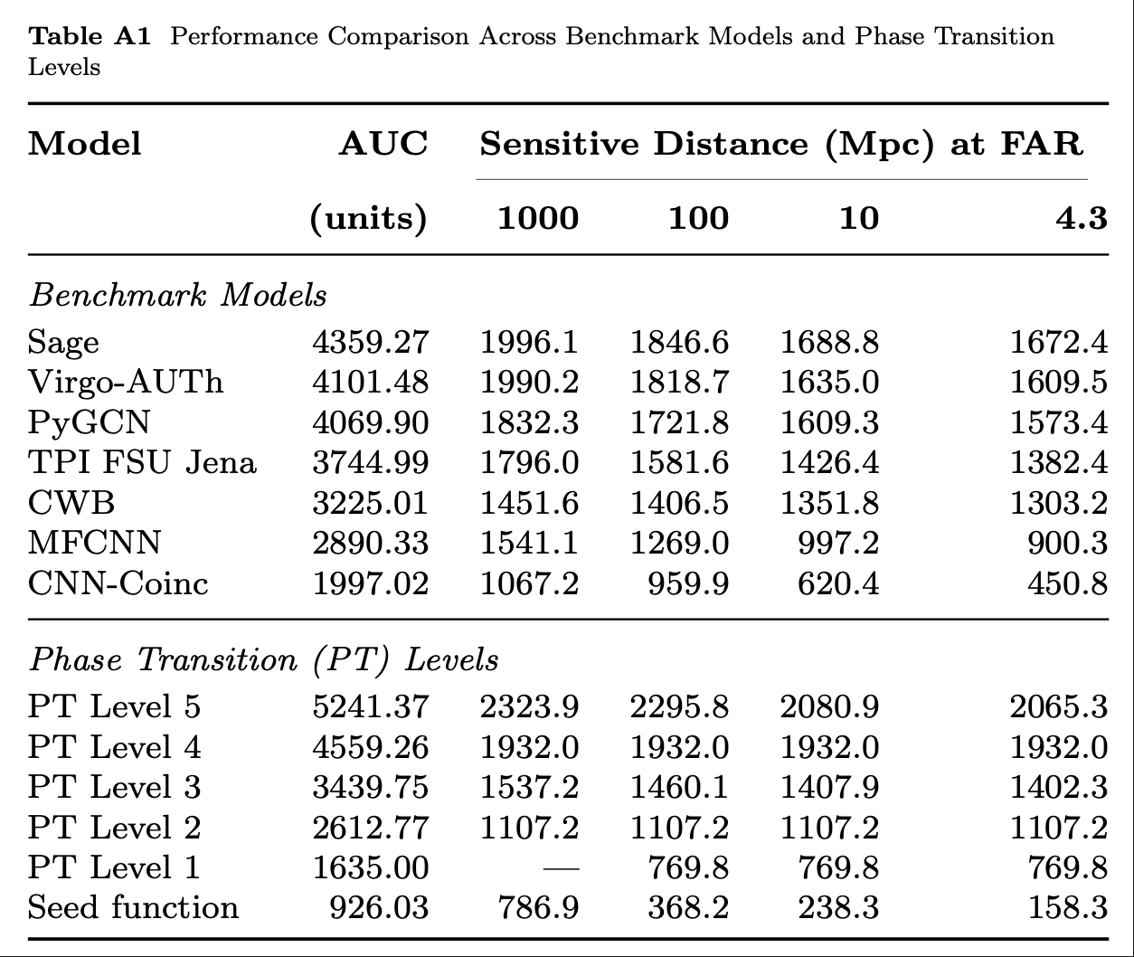
Automated exploration of algorithm parameter space
Benchmarking against state-of-the-art methods
hewang@ucas.ac.cn
HW & ZL, arXiv:2508.03661
Automated exploration of algorithm parameter space
Benchmarking against state-of-the-art methods
PyCBC (linear-core)
cWB (nonlinear-core)
Simple filters (non-linear)
CNN-like (highly non-linear)
20.2%
23.4%
hewang@ucas.ac.cn
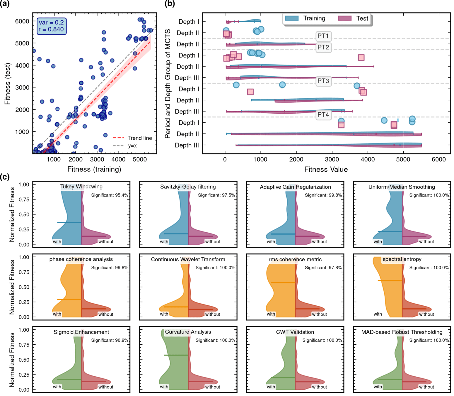
Algorithmic Component Impact Analysis.
import numpy as np
import scipy.signal as signal
from scipy.signal.windows import tukey
from scipy.signal import savgol_filter

def pipeline_v2(strain_h1: np.ndarray, strain_l1: np.ndarray, times: np.ndarray) -> tuple[np.ndarray, np.ndarray, np.ndarray]:
    """
    The pipeline function processes gravitational wave data from the H1 and L1 detectors to identify potential gravitational wave signals.
    It takes strain_h1 and strain_l1 numpy arrays containing detector data, and times array with corresponding time points.
    The function returns a tuple of three numpy arrays: peak_times containing GPS times of identified events,
    peak_heights with significance values of each peak, and peak_deltat showing time window uncertainty for each peak.
    """
    eps = np.finfo(float).tiny
    dt = times[1] - times[0]
    fs = 1.0 / dt
    # Base spectrogram parameters
    base_nperseg = 256
    base_noverlap = base_nperseg // 2
    medfilt_kernel = 101       # odd kernel size for robust detrending
    uncertainty_window = 5     # half-window for local timing uncertainty

    # -------------------- Stage 1: Robust Baseline Detrending --------------------
    # Remove long-term trends using a median filter for each channel.
    detrended_h1 = strain_h1 - signal.medfilt(strain_h1, kernel_size=medfilt_kernel)
    detrended_l1 = strain_l1 - signal.medfilt(strain_l1, kernel_size=medfilt_kernel)

    # -------------------- Stage 2: Adaptive Whitening with Enhanced PSD Smoothing --------------------
    def adaptive_whitening(strain: np.ndarray) -> np.ndarray:
        # Center the signal.
        centered = strain - np.mean(strain)
        n_samples = len(centered)
        # Adaptive window length: between 5 and 30 seconds
        win_length_sec = np.clip(n_samples / fs / 20, 5, 30)
        nperseg_adapt = int(win_length_sec * fs)
        nperseg_adapt = max(10, min(nperseg_adapt, n_samples))

        # Create a Tukey window with 75% overlap.
        tukey_alpha = 0.25
        win = tukey(nperseg_adapt, alpha=tukey_alpha)
        noverlap_adapt = int(nperseg_adapt * 0.75)
        if noverlap_adapt >= nperseg_adapt:
            noverlap_adapt = nperseg_adapt - 1

        # Estimate the power spectral density (PSD) using Welch's method.
        freqs, psd = signal.welch(centered, fs=fs, nperseg=nperseg_adapt,
                                  noverlap=noverlap_adapt, window=win, detrend='constant')
        psd = np.maximum(psd, eps)

        # Compute relative differences for PSD stationarity measure.
        diff_arr = np.abs(np.diff(psd)) / (psd[:-1] + eps)
        # Smooth the derivative with a moving average.
        if len(diff_arr) >= 3:
            smooth_diff = np.convolve(diff_arr, np.ones(3)/3, mode='same')
        else:
            smooth_diff = diff_arr

        # Exponential smoothing (Kalman-like) with adaptive alpha using PSD stationarity.
        smoothed_psd = np.copy(psd)
        for i in range(1, len(psd)):
            # Adaptive smoothing coefficient: base 0.8 modified by local stationarity (±0.05)
            local_alpha = np.clip(0.8 - 0.05 * smooth_diff[min(i-1, len(smooth_diff)-1)], 0.75, 0.85)
            smoothed_psd[i] = local_alpha * smoothed_psd[i-1] + (1 - local_alpha) * psd[i]

        # Compute Tikhonov regularization gain based on deviation from median PSD.
        noise_baseline = np.median(smoothed_psd)
        raw_gain = (smoothed_psd / (noise_baseline + eps)) - 1.0

        # Compute a causal-like gradient using the Savitzky-Golay filter.
        win_len = 11 if len(smoothed_psd) >= 11 else ((len(smoothed_psd)//2)*2+1)
        polyorder = 2 if win_len > 2 else 1
        delta_freq = np.mean(np.diff(freqs))
        grad_psd = savgol_filter(smoothed_psd, win_len, polyorder, deriv=1, delta=delta_freq, mode='interp')

        # Nonlinear scaling via sigmoid to enhance gradient differences.
        sigmoid = lambda x: 1.0 / (1.0 + np.exp(-x))
        scaling_factor = 1.0 + 2.0 * sigmoid(np.abs(grad_psd) / (np.median(smoothed_psd) + eps))

        # Compute adaptive gain factors with nonlinear scaling.
        gain = 1.0 - np.exp(-0.5 * scaling_factor * raw_gain)
        gain = np.clip(gain, -8.0, 8.0)

        # FFT-based whitening: interpolate gain and PSD onto FFT frequency bins.
        signal_fft = np.fft.rfft(centered)
        freq_bins = np.fft.rfftfreq(n_samples, d=dt)
        interp_gain = np.interp(freq_bins, freqs, gain, left=gain[0], right=gain[-1])
        interp_psd = np.interp(freq_bins, freqs, smoothed_psd, left=smoothed_psd[0], right=smoothed_psd[-1])
        denom = np.sqrt(interp_psd) * (np.abs(interp_gain) + eps)
        denom = np.maximum(denom, eps)
        white_fft = signal_fft / denom
        whitened = np.fft.irfft(white_fft, n=n_samples)
        return whitened

    # Whiten H1 and L1 channels using the adapted method.
    white_h1 = adaptive_whitening(detrended_h1)
    white_l1 = adaptive_whitening(detrended_l1)

    # -------------------- Stage 3: Coherent Time-Frequency Metric with Frequency-Conditioned Regularization --------------------
    def compute_coherent_metric(w1: np.ndarray, w2: np.ndarray) -> tuple[np.ndarray, np.ndarray]:
        # Compute complex spectrograms preserving phase information.
        f1, t_spec, Sxx1 = signal.spectrogram(w1, fs=fs, nperseg=base_nperseg,
                                              noverlap=base_noverlap, mode='complex', detrend=False)
        f2, t_spec2, Sxx2 = signal.spectrogram(w2, fs=fs, nperseg=base_nperseg,
                                               noverlap=base_noverlap, mode='complex', detrend=False)
        # Ensure common time axis length.
        common_len = min(len(t_spec), len(t_spec2))
        t_spec = t_spec[:common_len]
        Sxx1 = Sxx1[:, :common_len]
        Sxx2 = Sxx2[:, :common_len]

        # Compute phase differences and coherence between detectors.
        phase_diff = np.angle(Sxx1) - np.angle(Sxx2)
        phase_coherence = np.abs(np.cos(phase_diff))

        # Estimate median PSD per frequency bin from the spectrograms.
        psd1 = np.median(np.abs(Sxx1)**2, axis=1)
        psd2 = np.median(np.abs(Sxx2)**2, axis=1)

        # Frequency-conditioned regularization gain (reflection-guided).
        lambda_f = 0.5 * ((np.median(psd1) / (psd1 + eps)) + (np.median(psd2) / (psd2 + eps)))
        lambda_f = np.clip(lambda_f, 1e-4, 1e-2)
        # Regularization denominator integrating detector PSDs and lambda.
        reg_denom = (psd1[:, None] + psd2[:, None] + lambda_f[:, None] + eps)

        # Weighted phase coherence that balances phase alignment with noise levels.
        weighted_comp = phase_coherence / reg_denom

        # Compute axial (frequency) second derivatives as curvature estimates.
        d2_coh = np.gradient(np.gradient(phase_coherence, axis=0), axis=0)
        avg_curvature = np.mean(np.abs(d2_coh), axis=0)

        # Nonlinear activation boost using tanh for regions of high curvature.
        nonlinear_boost = np.tanh(5 * avg_curvature)
        linear_boost = 1.0 + 0.1 * avg_curvature

        # Cross-detector synergy: weight derived from global median consistency.
        novel_weight = np.mean((np.median(psd1) + np.median(psd2)) / (psd1[:, None] + psd2[:, None] + eps), axis=0)

        # Integrated time-frequency metric combining all enhancements.
        tf_metric = np.sum(weighted_comp * linear_boost * (1.0 + nonlinear_boost), axis=0) * novel_weight

        # Adjust the spectrogram time axis to account for window delay.
        metric_times = t_spec + times[0] + (base_nperseg / 2) / fs
        return tf_metric, metric_times

    tf_metric, metric_times = compute_coherent_metric(white_h1, white_l1)

    # -------------------- Stage 4: Multi-Resolution Thresholding with Octave-Spaced Dyadic Wavelet Validation --------------------
    def multi_resolution_thresholding(metric: np.ndarray, times_arr: np.ndarray) -> tuple[np.ndarray, np.ndarray, np.ndarray]:
        # Robust background estimation with median and MAD.
        bg_level = np.median(metric)
        mad_val = np.median(np.abs(metric - bg_level))
        robust_std = 1.4826 * mad_val
        threshold = bg_level + 1.5 * robust_std

        # Identify candidate peaks using prominence and minimum distance criteria.
        peaks, _ = signal.find_peaks(metric, height=threshold, distance=2, prominence=0.8 * robust_std)
        if peaks.size == 0:
            return np.array([]), np.array([]), np.array([])

        # Local uncertainty estimation using a Gaussian-weighted convolution.
        win_range = np.arange(-uncertainty_window, uncertainty_window + 1)
        sigma = uncertainty_window / 2.5
        gauss_kernel = np.exp(-0.5 * (win_range / sigma) ** 2)
        gauss_kernel /= np.sum(gauss_kernel)
        weighted_mean = np.convolve(metric, gauss_kernel, mode='same')
        weighted_sq = np.convolve(metric ** 2, gauss_kernel, mode='same')
        variances = np.maximum(weighted_sq - weighted_mean ** 2, 0.0)
        uncertainties = np.sqrt(variances)
        uncertainties = np.maximum(uncertainties, 0.01)

        valid_times = []
        valid_heights = []
        valid_uncerts = []
        n_metric = len(metric)

        # Compute a simple second derivative for local curvature checking.
        if n_metric > 2:
            second_deriv = np.diff(metric, n=2)
            second_deriv = np.pad(second_deriv, (1, 1), mode='edge')
        else:
            second_deriv = np.zeros_like(metric)

        # Use octave-spaced scales (dyadic wavelet validation) to validate peak significance.
        widths = np.arange(1, 9)  # approximate scales 1 to 8
        for peak in peaks:
            # Skip peaks lacking sufficient negative curvature.
            if second_deriv[peak] > -0.1 * robust_std:
                continue
            local_start = max(0, peak - uncertainty_window)
            local_end = min(n_metric, peak + uncertainty_window + 1)
            local_segment = metric[local_start:local_end]
            if len(local_segment) < 3:
                continue
            try:
                cwt_coeff = signal.cwt(local_segment, signal.ricker, widths)
            except Exception:
                continue
            max_coeff = np.max(np.abs(cwt_coeff))
            # Threshold for validating the candidate using local MAD.
            cwt_thresh = mad_val * np.sqrt(2 * np.log(len(local_segment) + eps))
            if max_coeff >= cwt_thresh:
                valid_times.append(times_arr[peak])
                valid_heights.append(metric[peak])
                valid_uncerts.append(uncertainties[peak])

        if len(valid_times) == 0:
            return np.array([]), np.array([]), np.array([])
        return np.array(valid_times), np.array(valid_heights), np.array(valid_uncerts)

    peak_times, peak_heights, peak_deltat = multi_resolution_thresholding(tf_metric, metric_times)
return peak_times, peak_heights, peak_deltatPT Level 5
HW & ZL, arXiv:2508.03661
PT Level 5
import numpy as np
import scipy.signal as signal
from scipy.signal.windows import tukey
from scipy.signal import savgol_filter

def pipeline_v2(strain_h1: np.ndarray, strain_l1: np.ndarray, times: np.ndarray) -> tuple[np.ndarray, np.ndarray, np.ndarray]:
    """
    The pipeline function processes gravitational wave data from the H1 and L1 detectors to identify potential gravitational wave signals.
    It takes strain_h1 and strain_l1 numpy arrays containing detector data, and times array with corresponding time points.
    The function returns a tuple of three numpy arrays: peak_times containing GPS times of identified events,
    peak_heights with significance values of each peak, and peak_deltat showing time window uncertainty for each peak.
    """
    eps = np.finfo(float).tiny
    dt = times[1] - times[0]
    fs = 1.0 / dt
    # Base spectrogram parameters
    base_nperseg = 256
    base_noverlap = base_nperseg // 2
    medfilt_kernel = 101       # odd kernel size for robust detrending
    uncertainty_window = 5     # half-window for local timing uncertainty

    # -------------------- Stage 1: Robust Baseline Detrending --------------------
    # Remove long-term trends using a median filter for each channel.
    detrended_h1 = strain_h1 - signal.medfilt(strain_h1, kernel_size=medfilt_kernel)
    detrended_l1 = strain_l1 - signal.medfilt(strain_l1, kernel_size=medfilt_kernel)

    # -------------------- Stage 2: Adaptive Whitening with Enhanced PSD Smoothing --------------------
    def adaptive_whitening(strain: np.ndarray) -> np.ndarray:
        # Center the signal.
        centered = strain - np.mean(strain)
        n_samples = len(centered)
        # Adaptive window length: between 5 and 30 seconds
        win_length_sec = np.clip(n_samples / fs / 20, 5, 30)
        nperseg_adapt = int(win_length_sec * fs)
        nperseg_adapt = max(10, min(nperseg_adapt, n_samples))

        # Create a Tukey window with 75% overlap.
        tukey_alpha = 0.25
        win = tukey(nperseg_adapt, alpha=tukey_alpha)
        noverlap_adapt = int(nperseg_adapt * 0.75)
        if noverlap_adapt >= nperseg_adapt:
            noverlap_adapt = nperseg_adapt - 1

        # Estimate the power spectral density (PSD) using Welch's method.
        freqs, psd = signal.welch(centered, fs=fs, nperseg=nperseg_adapt,
                                  noverlap=noverlap_adapt, window=win, detrend='constant')
        psd = np.maximum(psd, eps)

        # Compute relative differences for PSD stationarity measure.
        diff_arr = np.abs(np.diff(psd)) / (psd[:-1] + eps)
        # Smooth the derivative with a moving average.
        if len(diff_arr) >= 3:
            smooth_diff = np.convolve(diff_arr, np.ones(3)/3, mode='same')
        else:
            smooth_diff = diff_arr

        # Exponential smoothing (Kalman-like) with adaptive alpha using PSD stationarity.
        smoothed_psd = np.copy(psd)
        for i in range(1, len(psd)):
            # Adaptive smoothing coefficient: base 0.8 modified by local stationarity (±0.05)
            local_alpha = np.clip(0.8 - 0.05 * smooth_diff[min(i-1, len(smooth_diff)-1)], 0.75, 0.85)
            smoothed_psd[i] = local_alpha * smoothed_psd[i-1] + (1 - local_alpha) * psd[i]

        # Compute Tikhonov regularization gain based on deviation from median PSD.
        noise_baseline = np.median(smoothed_psd)
        raw_gain = (smoothed_psd / (noise_baseline + eps)) - 1.0

        # Compute a causal-like gradient using the Savitzky-Golay filter.
        win_len = 11 if len(smoothed_psd) >= 11 else ((len(smoothed_psd)//2)*2+1)
        polyorder = 2 if win_len > 2 else 1
        delta_freq = np.mean(np.diff(freqs))
        grad_psd = savgol_filter(smoothed_psd, win_len, polyorder, deriv=1, delta=delta_freq, mode='interp')

        # Nonlinear scaling via sigmoid to enhance gradient differences.
        sigmoid = lambda x: 1.0 / (1.0 + np.exp(-x))
        scaling_factor = 1.0 + 2.0 * sigmoid(np.abs(grad_psd) / (np.median(smoothed_psd) + eps))

        # Compute adaptive gain factors with nonlinear scaling.
        gain = 1.0 - np.exp(-0.5 * scaling_factor * raw_gain)
        gain = np.clip(gain, -8.0, 8.0)

        # FFT-based whitening: interpolate gain and PSD onto FFT frequency bins.
        signal_fft = np.fft.rfft(centered)
        freq_bins = np.fft.rfftfreq(n_samples, d=dt)
        interp_gain = np.interp(freq_bins, freqs, gain, left=gain[0], right=gain[-1])
        interp_psd = np.interp(freq_bins, freqs, smoothed_psd, left=smoothed_psd[0], right=smoothed_psd[-1])
        denom = np.sqrt(interp_psd) * (np.abs(interp_gain) + eps)
        denom = np.maximum(denom, eps)
        white_fft = signal_fft / denom
        whitened = np.fft.irfft(white_fft, n=n_samples)
        return whitened

    # Whiten H1 and L1 channels using the adapted method.
    white_h1 = adaptive_whitening(detrended_h1)
    white_l1 = adaptive_whitening(detrended_l1)

    # -------------------- Stage 3: Coherent Time-Frequency Metric with Frequency-Conditioned Regularization --------------------
    def compute_coherent_metric(w1: np.ndarray, w2: np.ndarray) -> tuple[np.ndarray, np.ndarray]:
        # Compute complex spectrograms preserving phase information.
        f1, t_spec, Sxx1 = signal.spectrogram(w1, fs=fs, nperseg=base_nperseg,
                                              noverlap=base_noverlap, mode='complex', detrend=False)
        f2, t_spec2, Sxx2 = signal.spectrogram(w2, fs=fs, nperseg=base_nperseg,
                                               noverlap=base_noverlap, mode='complex', detrend=False)
        # Ensure common time axis length.
        common_len = min(len(t_spec), len(t_spec2))
        t_spec = t_spec[:common_len]
        Sxx1 = Sxx1[:, :common_len]
        Sxx2 = Sxx2[:, :common_len]

        # Compute phase differences and coherence between detectors.
        phase_diff = np.angle(Sxx1) - np.angle(Sxx2)
        phase_coherence = np.abs(np.cos(phase_diff))

        # Estimate median PSD per frequency bin from the spectrograms.
        psd1 = np.median(np.abs(Sxx1)**2, axis=1)
        psd2 = np.median(np.abs(Sxx2)**2, axis=1)

        # Frequency-conditioned regularization gain (reflection-guided).
        lambda_f = 0.5 * ((np.median(psd1) / (psd1 + eps)) + (np.median(psd2) / (psd2 + eps)))
        lambda_f = np.clip(lambda_f, 1e-4, 1e-2)
        # Regularization denominator integrating detector PSDs and lambda.
        reg_denom = (psd1[:, None] + psd2[:, None] + lambda_f[:, None] + eps)

        # Weighted phase coherence that balances phase alignment with noise levels.
        weighted_comp = phase_coherence / reg_denom

        # Compute axial (frequency) second derivatives as curvature estimates.
        d2_coh = np.gradient(np.gradient(phase_coherence, axis=0), axis=0)
        avg_curvature = np.mean(np.abs(d2_coh), axis=0)

        # Nonlinear activation boost using tanh for regions of high curvature.
        nonlinear_boost = np.tanh(5 * avg_curvature)
        linear_boost = 1.0 + 0.1 * avg_curvature

        # Cross-detector synergy: weight derived from global median consistency.
        novel_weight = np.mean((np.median(psd1) + np.median(psd2)) / (psd1[:, None] + psd2[:, None] + eps), axis=0)

        # Integrated time-frequency metric combining all enhancements.
        tf_metric = np.sum(weighted_comp * linear_boost * (1.0 + nonlinear_boost), axis=0) * novel_weight

        # Adjust the spectrogram time axis to account for window delay.
        metric_times = t_spec + times[0] + (base_nperseg / 2) / fs
        return tf_metric, metric_times

    tf_metric, metric_times = compute_coherent_metric(white_h1, white_l1)

    # -------------------- Stage 4: Multi-Resolution Thresholding with Octave-Spaced Dyadic Wavelet Validation --------------------
    def multi_resolution_thresholding(metric: np.ndarray, times_arr: np.ndarray) -> tuple[np.ndarray, np.ndarray, np.ndarray]:
        # Robust background estimation with median and MAD.
        bg_level = np.median(metric)
        mad_val = np.median(np.abs(metric - bg_level))
        robust_std = 1.4826 * mad_val
        threshold = bg_level + 1.5 * robust_std

        # Identify candidate peaks using prominence and minimum distance criteria.
        peaks, _ = signal.find_peaks(metric, height=threshold, distance=2, prominence=0.8 * robust_std)
        if peaks.size == 0:
            return np.array([]), np.array([]), np.array([])

        # Local uncertainty estimation using a Gaussian-weighted convolution.
        win_range = np.arange(-uncertainty_window, uncertainty_window + 1)
        sigma = uncertainty_window / 2.5
        gauss_kernel = np.exp(-0.5 * (win_range / sigma) ** 2)
        gauss_kernel /= np.sum(gauss_kernel)
        weighted_mean = np.convolve(metric, gauss_kernel, mode='same')
        weighted_sq = np.convolve(metric ** 2, gauss_kernel, mode='same')
        variances = np.maximum(weighted_sq - weighted_mean ** 2, 0.0)
        uncertainties = np.sqrt(variances)
        uncertainties = np.maximum(uncertainties, 0.01)

        valid_times = []
        valid_heights = []
        valid_uncerts = []
        n_metric = len(metric)

        # Compute a simple second derivative for local curvature checking.
        if n_metric > 2:
            second_deriv = np.diff(metric, n=2)
            second_deriv = np.pad(second_deriv, (1, 1), mode='edge')
        else:
            second_deriv = np.zeros_like(metric)

        # Use octave-spaced scales (dyadic wavelet validation) to validate peak significance.
        widths = np.arange(1, 9)  # approximate scales 1 to 8
        for peak in peaks:
            # Skip peaks lacking sufficient negative curvature.
            if second_deriv[peak] > -0.1 * robust_std:
                continue
            local_start = max(0, peak - uncertainty_window)
            local_end = min(n_metric, peak + uncertainty_window + 1)
            local_segment = metric[local_start:local_end]
            if len(local_segment) < 3:
                continue
            try:
                cwt_coeff = signal.cwt(local_segment, signal.ricker, widths)
            except Exception:
                continue
            max_coeff = np.max(np.abs(cwt_coeff))
            # Threshold for validating the candidate using local MAD.
            cwt_thresh = mad_val * np.sqrt(2 * np.log(len(local_segment) + eps))
            if max_coeff >= cwt_thresh:
                valid_times.append(times_arr[peak])
                valid_heights.append(metric[peak])
                valid_uncerts.append(uncertainties[peak])

        if len(valid_times) == 0:
            return np.array([]), np.array([]), np.array([])
        return np.array(valid_times), np.array(valid_heights), np.array(valid_uncerts)

    peak_times, peak_heights, peak_deltat = multi_resolution_thresholding(tf_metric, metric_times)
return peak_times, peak_heights, peak_deltatHW & ZL, arXiv:2508.03661
Out-of-distribution (OOD) detection
hewang@ucas.ac.cn
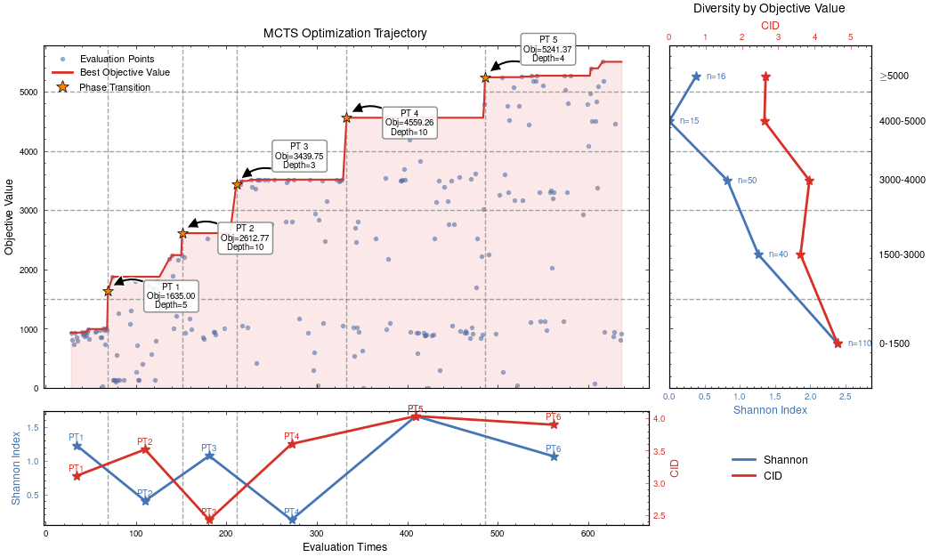
MCTS Depth-Stratified Performance Analysis.
Algorithmic Component Impact Analysis.
HW & ZL, arXiv:2508.03661
hewang@ucas.ac.cn
Algorithmic Component Impact Analysis.
HW & ZL, arXiv:2508.03661
Please analyze the following Python code snippet for gravitational wave detection and
extract technical features in JSON format.

The code typically has three main stages:
1. Data Conditioning: preprocessing, filtering, whitening, etc.
2. Time-Frequency Analysis: spectrograms, FFT, wavelets, etc.
3. Trigger Analysis: peak detection, thresholding, validation, etc.

For each stage present in the code, extract:
- Technical methods used
- Libraries and functions called
- Algorithm complexity features
- Key parameters

Code to analyze:
```python
{code_snippet}
```

Please return a JSON object with this structure:
{
  "algorithm_id": "{algorithm_id}",
  "stages": {
    "data_conditioning": {
      "present": true/false,
      "techniques": ["technique1", "technique2"],
      "libraries": ["lib1", "lib2"],
      "functions": ["func1", "func2"],
      "parameters": {"param1": "value1"},
      "complexity": "low/medium/high"
    },
    "time_frequency_analysis": {...},
    "trigger_analysis": {...}
  },
  "overall_complexity": "low/medium/high",
  "total_lines": 0,
  "unique_libraries": ["lib1", "lib2"],
  "code_quality_score": 0.0
}

Only return the JSON object, no additional text.
hewang@ucas.ac.cn
HW & ZL, arXiv:2508.03661
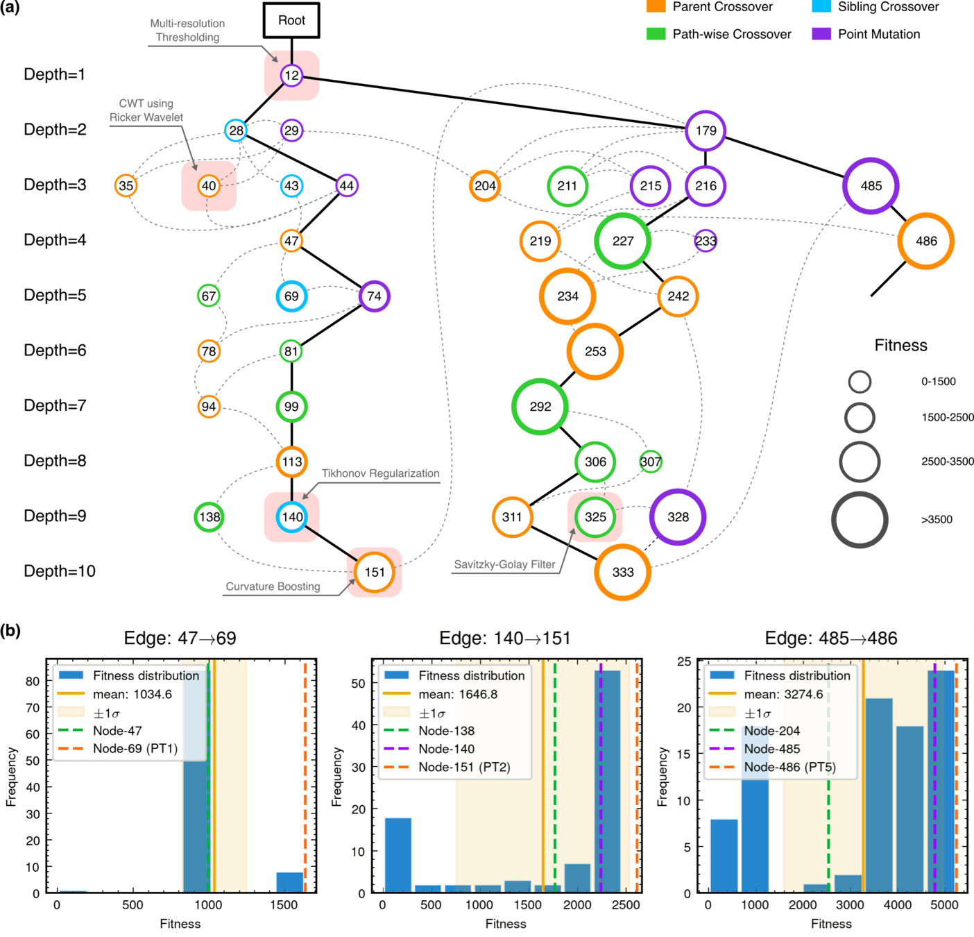
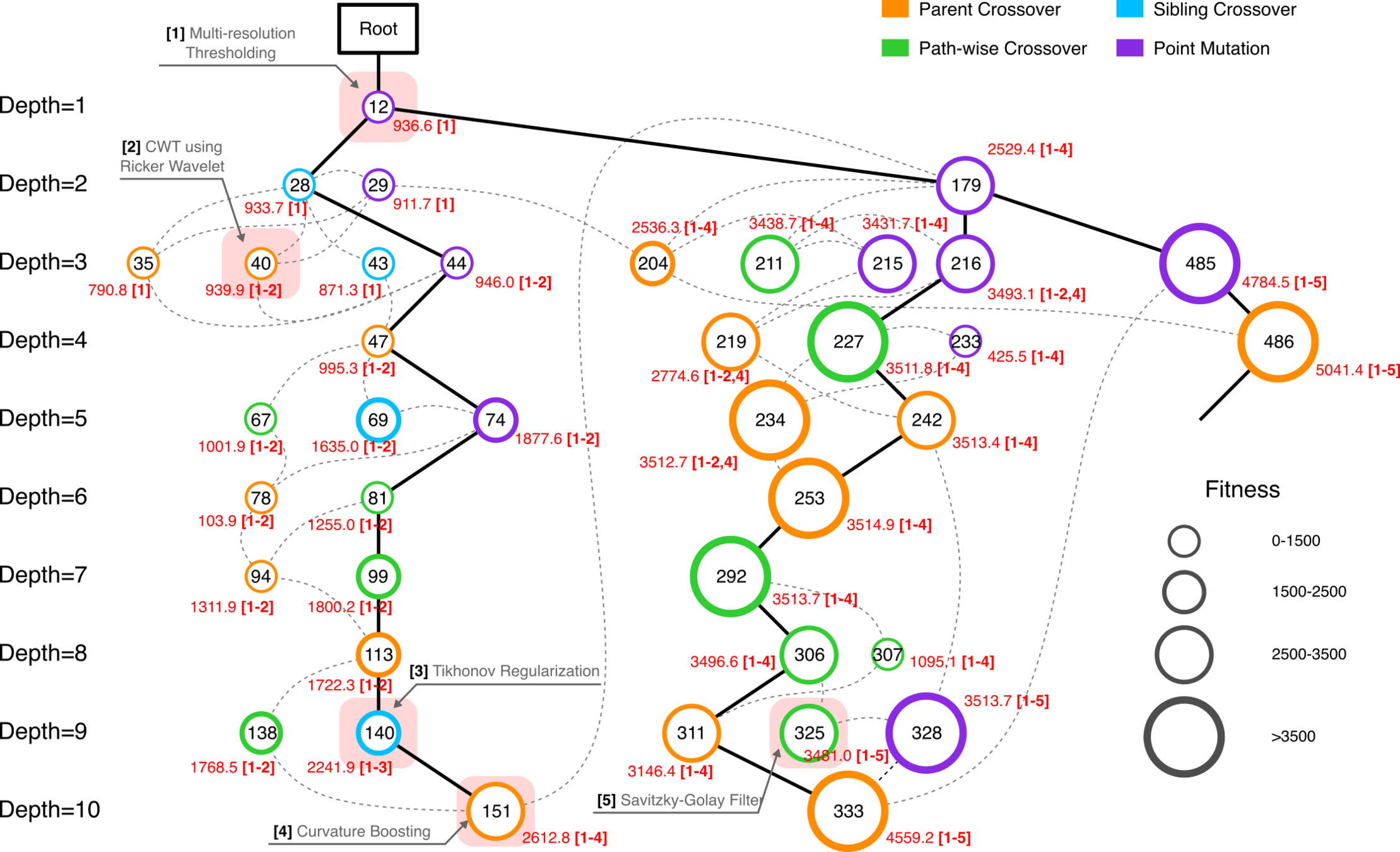
MCTS Algorithmic Evolution Pathway
hewang@ucas.ac.cn
HW & ZL, arXiv:2508.03661
MCTS Algorithmic Evolution Pathway
hewang@ucas.ac.cn
HW & ZL, arXiv:2508.03661
52.8% achieving superior fitness with 100% Tikhonov regularization inheritance
89.3% variants exceeding preceding node performance
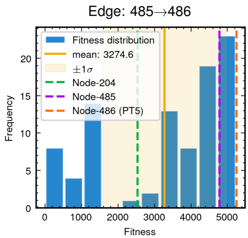
70.7% variants outperforming node 204, 25.0% surpassing node 485
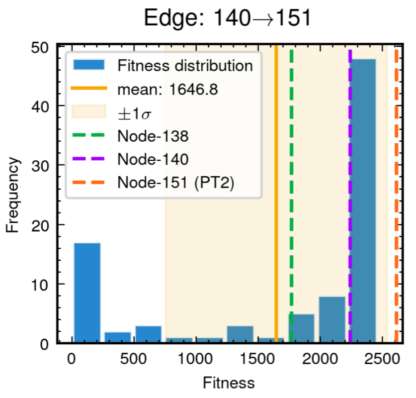
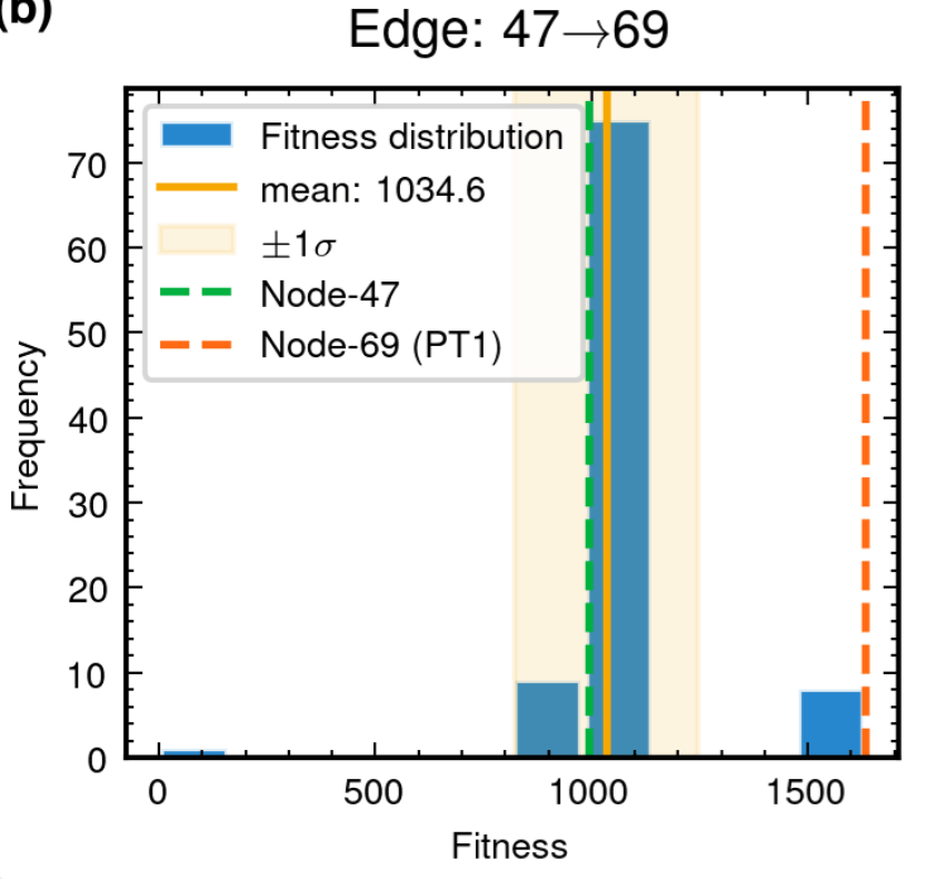
Edge robustness analysis for three critical evolutionary transitions.
hewang@ucas.ac.cn
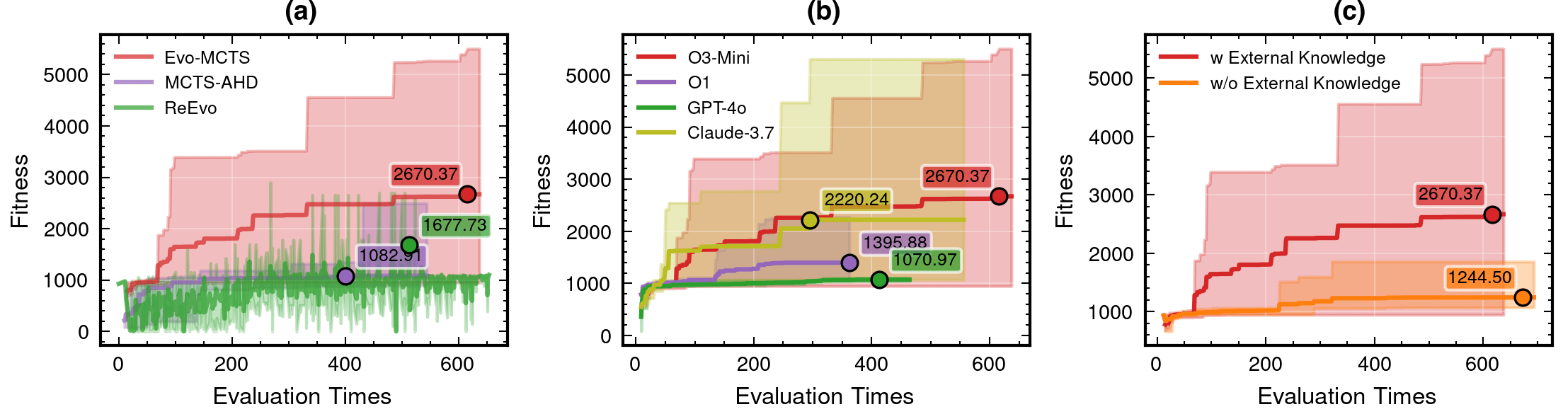
Integrated Architecture Validation
Contributions of knowledge synthesis
LLM Model Selection and Robustness Analysis
o3-mini-medium
o1-2024-12-17
gpt-4o-2024-11-20
claude-3-7-sonnet-20250219-thinking
59.1%
MCTS-AHD (2501.08603)
ReEvo (2402.01145)
HW & ZL, arXiv:2508.03661
hewang@ucas.ac.cn
Integrated Architecture Validation
Contributions of knowledge synthesis
LLM Model Selection and Robustness Analysis
o3-mini-medium
o1-2024-12-17
gpt-4o-2024-11-20
claude-3-7-sonnet-20250219-thinking
59.1%
HW & ZL, arXiv:2508.03661
hewang@ucas.ac.cn
Integrated Architecture Validation
Contributions of knowledge synthesis
59.1%
HW & ZL, arXiv:2508.03661
### External Knowledge Integration
1. **Non-linear** Processing Core Concepts:
    - Signal Transformation:
        * Non-linear vs linear decomposition
        * Adaptive threshold mechanisms
        * Multi-scale analysis

    - Feature Extraction:
        * Phase space reconstruction
        * Topological data analysis
        * Wavelet-based detection

    - Statistical Analysis:
        * Robust estimators
        * Non-Gaussian processes
        * Higher-order statistics

2. Implementation Principles:
    - Prioritize adaptive over fixed parameters
    - Consider local vs global characteristics
- Balance computational cost with accuracyhewang@ucas.ac.cn
Key Challenge: How can we maintain the interpretability advantages of traditional models while leveraging the power of AI approaches?
Key Trust Factors:
Motivation 1: Traditional methods heavily rely on manually designed filters and statistics.
Motivation 2: AI interpretability challenge: Discoveries vs. Validation.
Traditional Physics Approach
Input
Human-Designed Algorithm
(Based on human insight)
Output
Example: Matched Filtering, linear regression
Data/
Experience
Black-Box AI Approach
Input
AI Model
(Low interpretability)
Output
Examples: CNN, AlphaGo, DINGO
Data/
Experience
hewang@ucas.ac.cn
Black-Box AI Approach
Input
AI Model
(Low interpretability)
Output
Examples: CNN, AlphaGo, DINGO
Traditional Physics Approach
Input
Human-Designed Algorithm
(Based on human insight)
Output
Example: Matched Filtering, linear regression
Data/
Experience
Data/
Experience
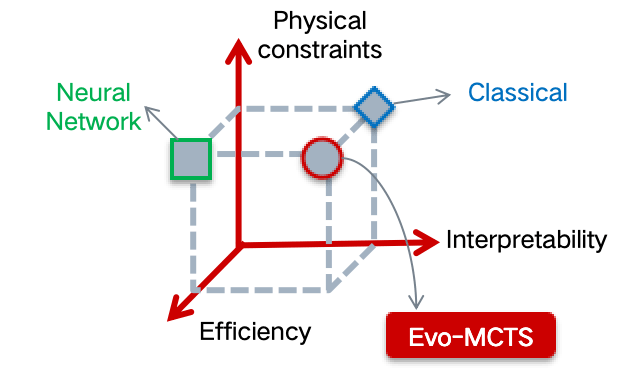
Our Mission: To create transparent AI systems that combine physics-based interpretability with deep learning capabilities
Interpretable AI Approach
The best of both worlds
Input
Physics-Informed
Algorithm
(High interpretability)
Output
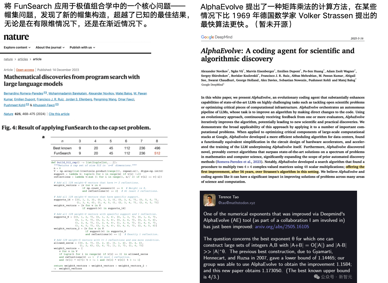
Example: Evo-MCTS, AlphaEvolve
Physics
Knowledge
AI Model
🎯 OUR WORK
Motivation 1: Traditional methods heavily rely on manually designed filters and statistics.
Motivation 2: AI interpretability challenge: Discoveries vs. Validation.
hewang@ucas.ac.cn
Any algorithm's design problem can be viewed as an optimization challenge
FYI:
hewang@ucas.ac.cn
HW & ZL, arXiv:2508.03661
Automated exploration of algorithm parameter space
Benchmarking against state-of-the-art methods
PyCBC (linear-core)
cWB (nonlinear-core)
Simple filters (non-linear)
CNN-like (highly non-linear)
Black-Box AI Approach
Input
AI Model
(Low interpretability)
Output
Examples: CNN, AlphaGo, DINGO
Traditional Physics Approach
Input
Human-Designed Algorithm
(Based on human insight)
Output
Example: Matched Filtering, linear regression
Data/
Experience
Data/
Experience
Our Mission: To create transparent AI systems that combine physics-based interpretability with deep learning capabilities
Interpretable AI Approach
The best of both worlds
Input
Physics-Informed
Algorithm
(High interpretability)
Output
Example: Evo-MCTS (ours), AlphaEvolve
Physics
Knowledge
AI Model
🎯 OUR WORK
Who Am I
— A quick intro and how I got into this field
What Is Machine Learning?
— The basics and why it matters
Deep Learning: When Machines Start to See and Think
— From neural networks to powerful representations
Gravitational Waves Meet Machine Learning
— How ML is reshaping data analysis in GW astronomy
Let’s Get Practical: Searching for Gravitational Waves
— A hands-on look at applying ML in real GW searches
LLMs for Gravitational Waves: My Ongoing Work
— Towards automated and interpretable scientific discovery
for _ in range(num_of_audiences):
    print('Thank you for your attention! 🙏')
hewang@ucas.ac.cn
Acknowledgment:
This slide: https://slides.com/iphysresearch/2025nov_fqcp
Who Am I
— A quick intro and how I got into this field
What Is Machine Learning?
— The basics and why it matters
Deep Learning: When Machines Start to See and Think
— From neural networks to powerful representations
Gravitational Waves Meet Machine Learning
— How ML is reshaping data analysis in GW astronomy
Let’s Get Practical: Searching for Gravitational Waves
— A hands-on look at applying ML in real GW searches
LLMs for Gravitational Waves: My Ongoing Work
— Towards automated and interpretable scientific discovery
hewang@ucas.ac.cn
# GW: DL
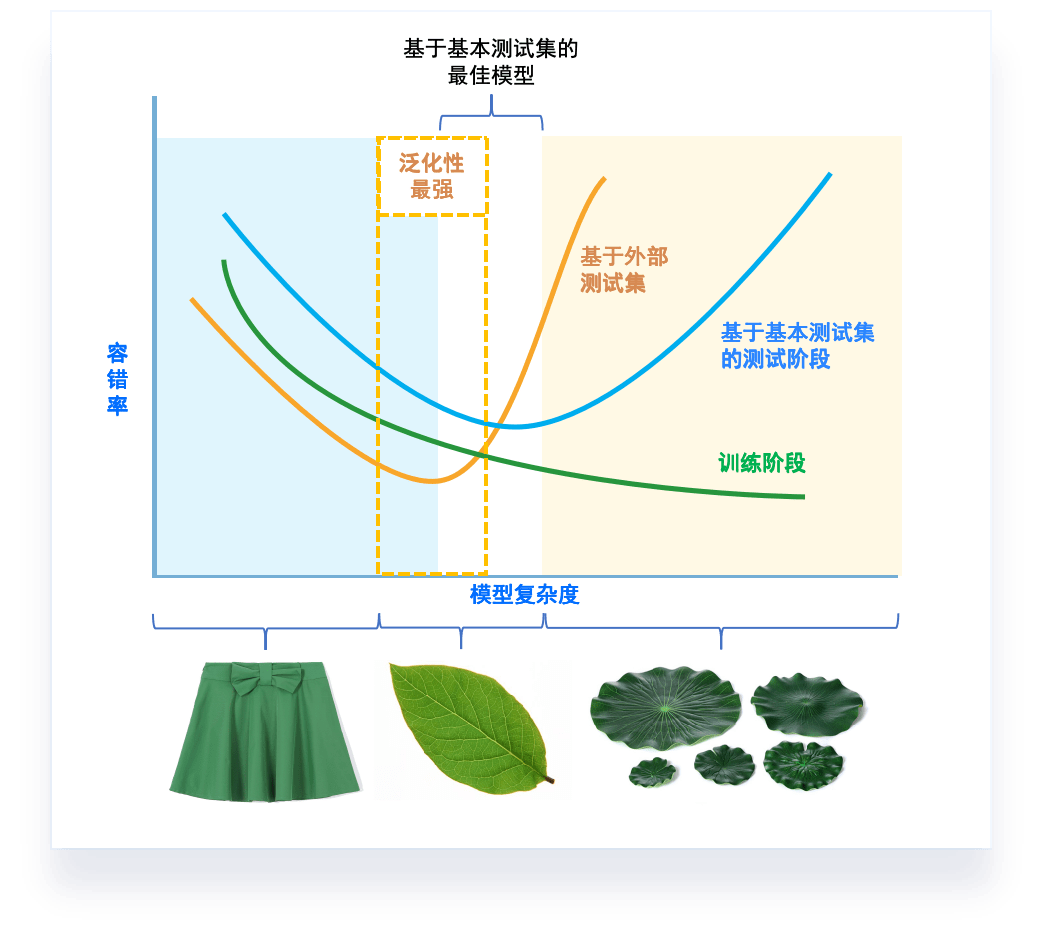
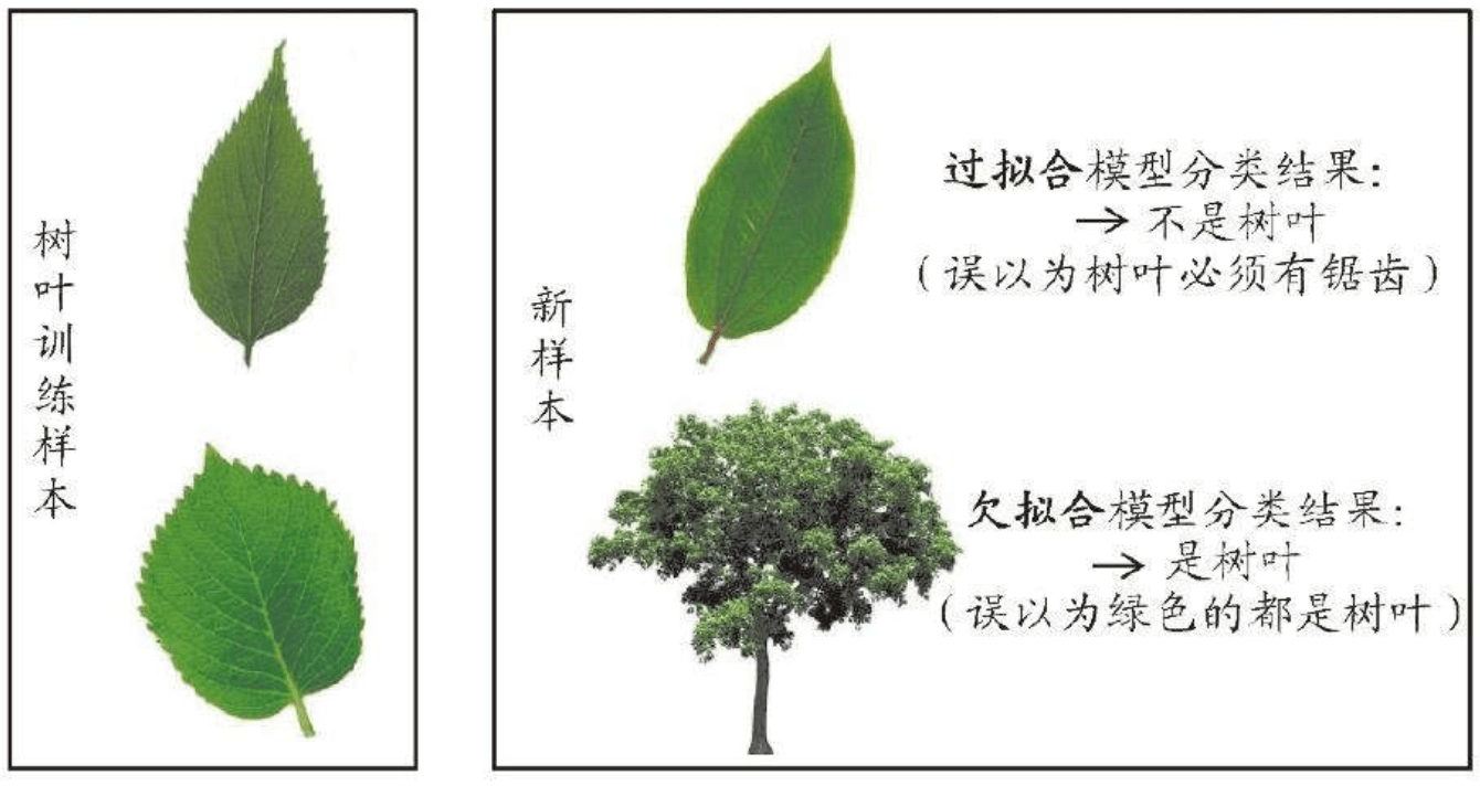
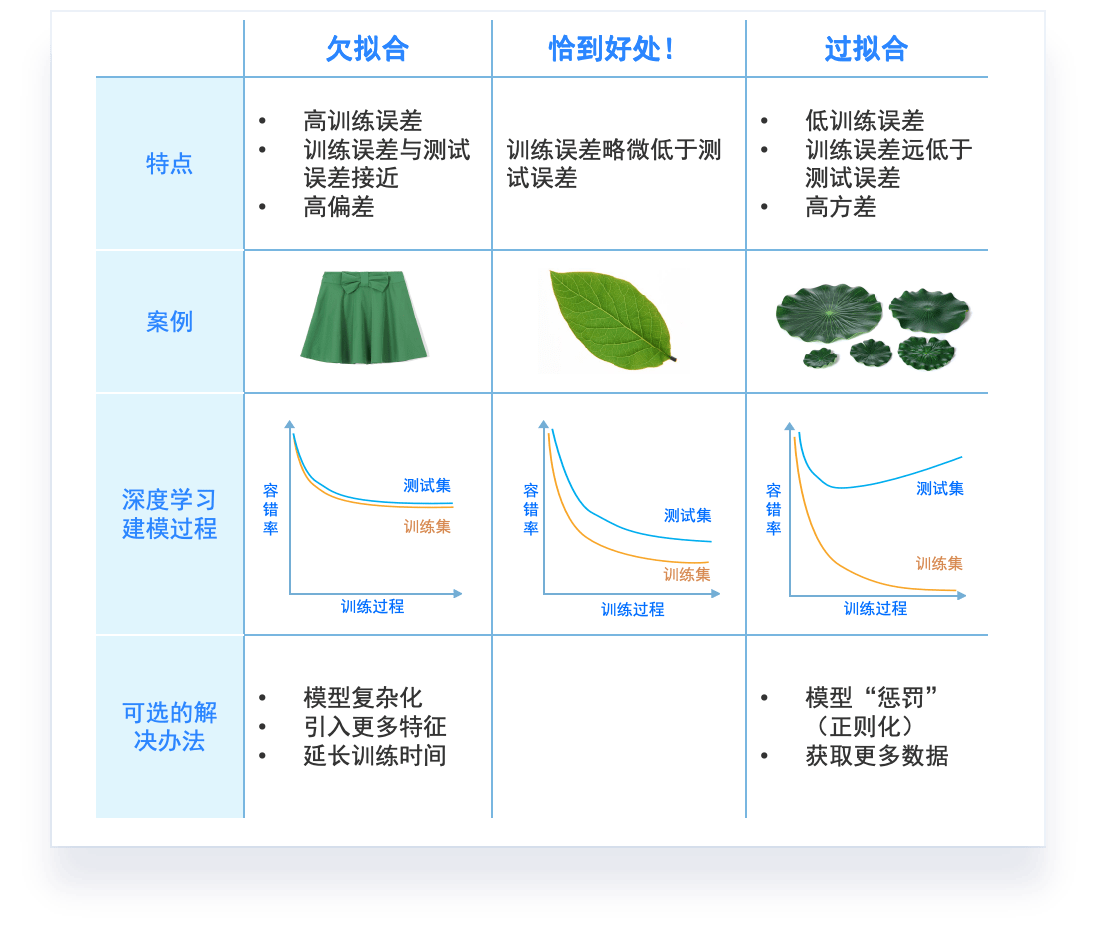
模型调优,过拟合与欠拟合
# GW: DL
模型调优,过拟合与欠拟合
# GW: DL
模型调优,过拟合与欠拟合
素材来源:DOI: 10.1177/2374289519873088
# GW: DL
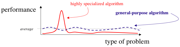
没有免费午餐定理(No free lunch theorem)
Wolpert D H. The lack of a priori distinctions between learning algorithms[J]. Neural computation, 1996, 8(7): 1341-1390.
没有免费午餐理论对于个人的指导
# GW: DL
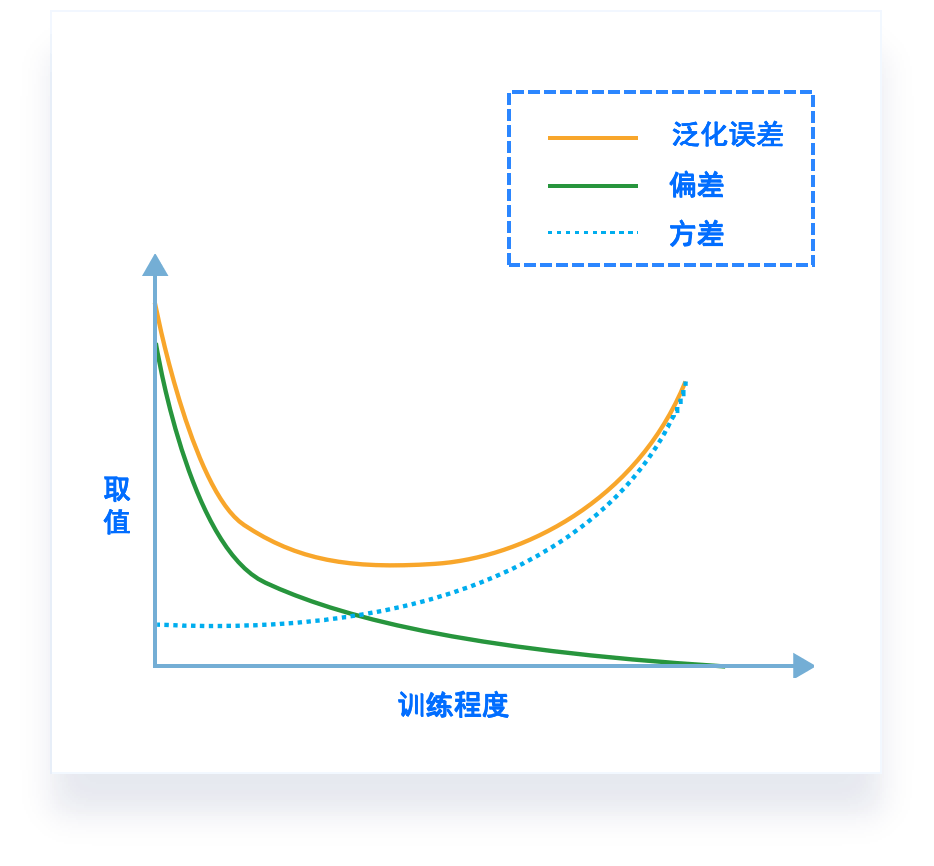
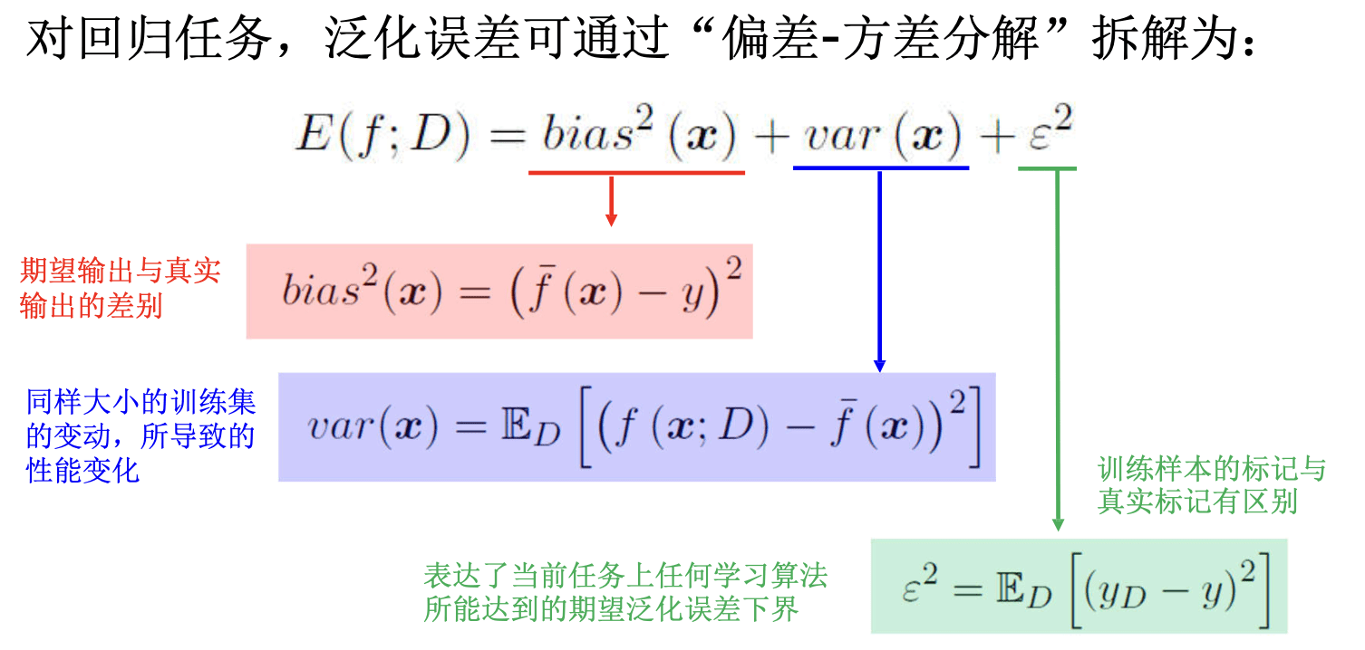
偏差-方差窘境(bias-variance dilemma)
泛化性能 是由学习算法的能力、数据的充分性以及学习任务本身的难度共同决定。
# GW: DL
模型调优,过拟合与欠拟合
过拟合和欠拟合是机器学习中常见的两种问题。
# GW: DL
模型评估与选择
统计假设检验 (hypothesis test) 为学习器性能比较提供了重要依据【应需要有统计显著性作为评判依据】
两学习器比较
交叉验证 t 检验(基于成对 t 检验)
McNemar 检验(基于列联表、卡方检验)
多学习器比较
Kolmogorv-Smirnov Test (K-S检验)
Friedman 检验 (基于序值,F检验;判断“是否相同”)
Nemenyi 后续检验(基于序值,进一步判断两两差别)
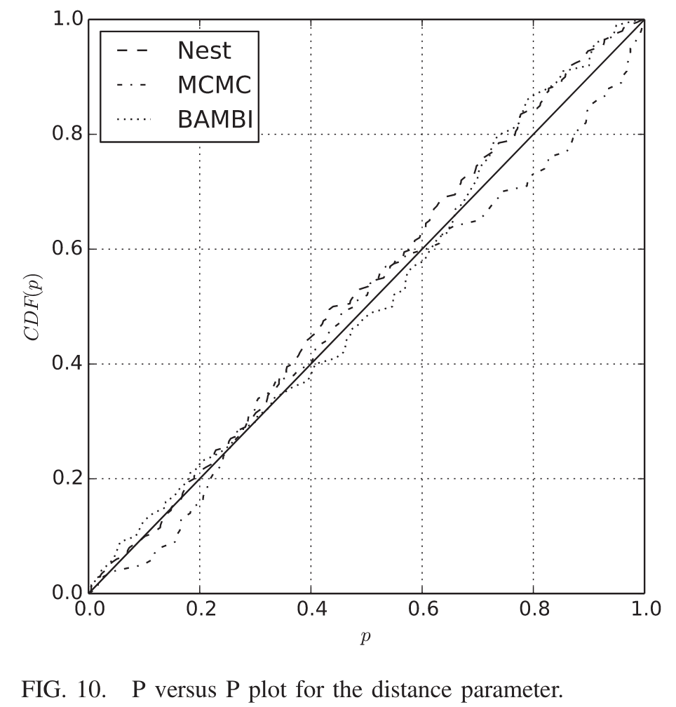
Veitch, J., et al. Physical Review D 91, no. 4 (February 2015): 042003. https://doi.org/10.1103/PhysRevD.91.042003.
By He Wang
11.13.2025 @FQCP2025 (https://indico.ictp-ap.ucas.ac.cn/event/4/https://indico.ictp-ap.ucas.ac.cn/event/4/


