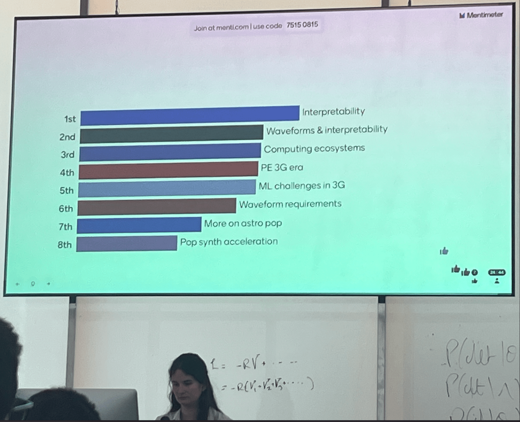
He Wang

hewang@ucas.ac.cn

University of Chinese Academy of Sciences (UCAS)

on behalf of KAGRA collaboration

Nature Conferences: "AI for Discovery and Research Automation" on 17th October 2025

Based on arXiv:2508.03661

LLM-Guided Evolutionary Monte Carlo Tree Search for Explainable Algorithm Discovery in Gravitational-Wave Detection

动机1：传统方法严重依赖人工经验构造滤波器与统计量

动机2：AI 可解释性挑战: Discoveries vs. Validation

He Wang | ICTP-AP, UCAS

hewang@ucas.ac.cn

Motivation I: Rely on Experience for Filters and Statistics

He Wang | ICTP-AP, UCAS

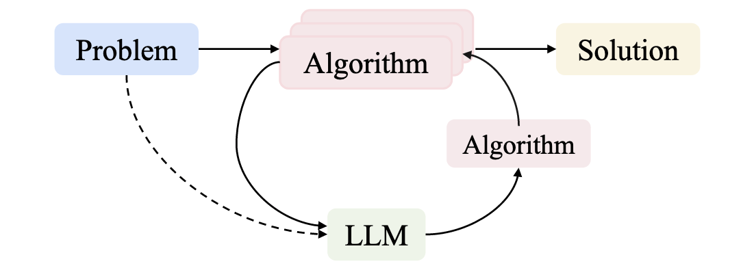
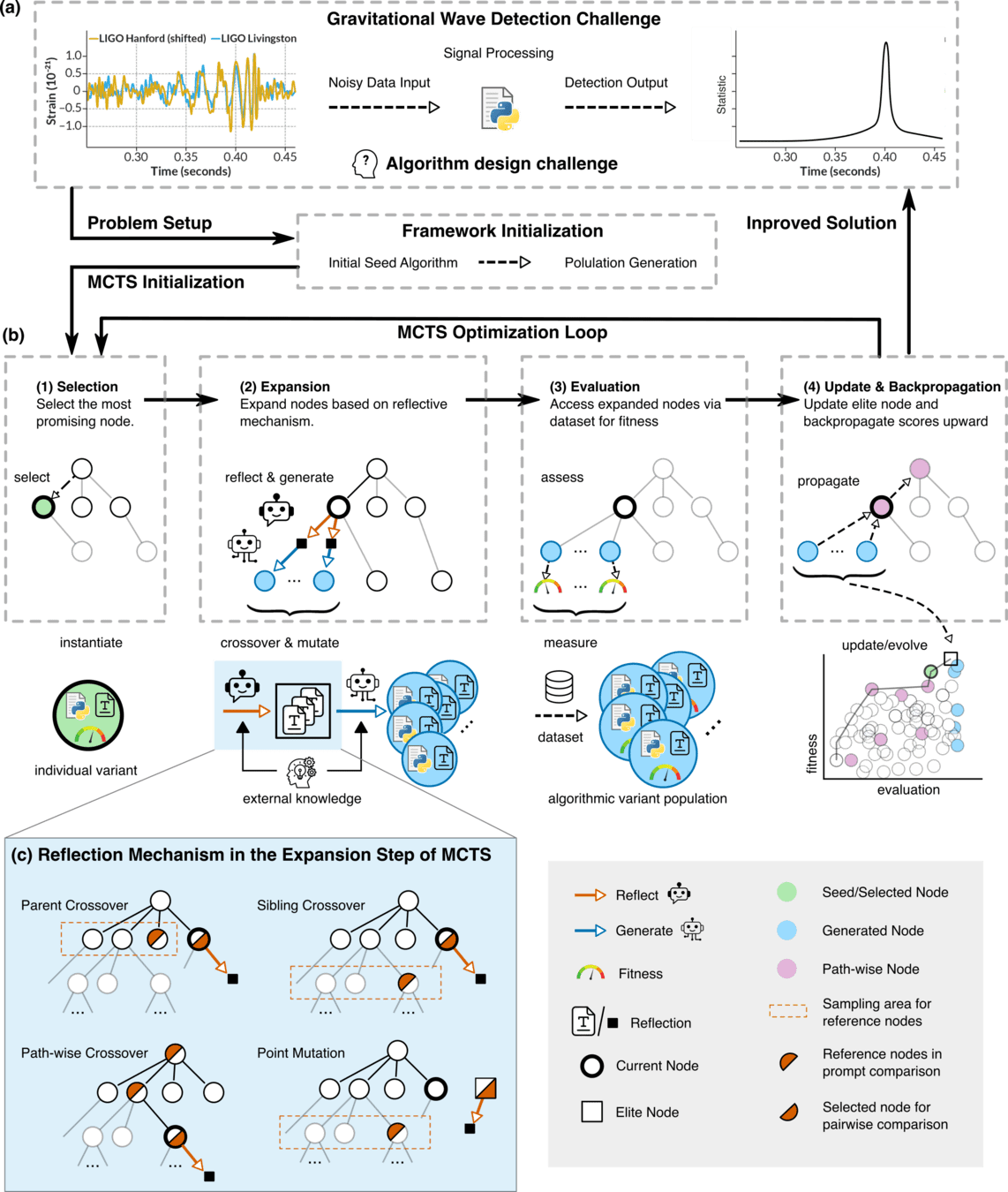
AAD for GW detection Guided by LLM-informed Evo-MCTS

h_w[t]

d_w[t]

\rho[t]

Linear Filter

Input Series

Output Series

h_w[t]

Impulse Response:

Digital Signal Processing Approach

Nitz et al., ApJ (2017)

Matched Filtering Techniques

In Gaussian and stationary noise environments, the optimal linear algorithm for extracting weak signals
Works by correlating a known signal model \(h(t)\) (template) with the data.
Starting with data: \(d(t) = h(t) + n(t)\).
Defining the matched-filtering SNR \(\rho(t)\):
\(\rho^2(t)\equiv\frac{1}{\langle h|h \rangle}|\langle d|h \rangle(t)|^2 \) , where
\(\langle d|h \rangle (t) = 4\int^\infty_0\frac{\tilde{d}(f)\tilde{h}^*(f)}{S_n(f)}e^{2\pi ift}df \) ,
\(\langle h|h \rangle = 4\int^\infty_0\frac{\tilde{h}(f)\tilde{h}^*(f)}{S_n(f)}df \),
\(S_n(f)\) is noise power spectral density (one-sided).

Statistical Approaches

Frequentist Testing:

Make assumptions about signal and noise
Write down the likelihood function
Maximize parameters
Define detection statistic
→ recover MF

Bayesian Testing:

Start from same likelihood
Define parameter priors
Marginalize over parameters
Often treated as Frequentist statistic
→ recover MF (for certain priors)

He Wang | ICTP-AP, UCAS

hewang@ucas.ac.cn

He Wang | ICTP-AP, UCAS

AAD for GW detection Guided by LLM-informed Evo-MCTS

Motivation I: Linear template method using prior data

Traditional matching filters need large templates, increasing computational costs and noise sensitivity, which hampers new gravitational wave signal detection.

Motivation II: Black-box data-driven learning methods

Deep neural networks excel in nonlinear modeling but are "black boxes" with poor interpretability, making them unsuitable for high-risk scientific validation.

The strict requirements for algorithm discovery

Physical constraints: Must follow physical laws and domain knowledge
Efficiency: Must navigate large, costly search spaces
Interpretability: Must be understandable and verifiable by experts

Large Language Models (LLMs) as Designers

LLMs are used in Automated Algorithmic Discovery (AAD) to directly create algorithms or specific components, which are commonly incorporated iteratively to continuously search for better designs.

external_knowledge
(constraint)

Fitness

Challenges and Motivations

He Wang | ICTP-AP, UCAS

Motivation II: AI Interpretability Challenges: Discoveries vs. Validation

hewang@ucas.ac.cn

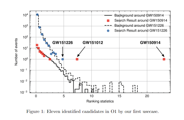
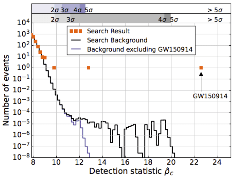
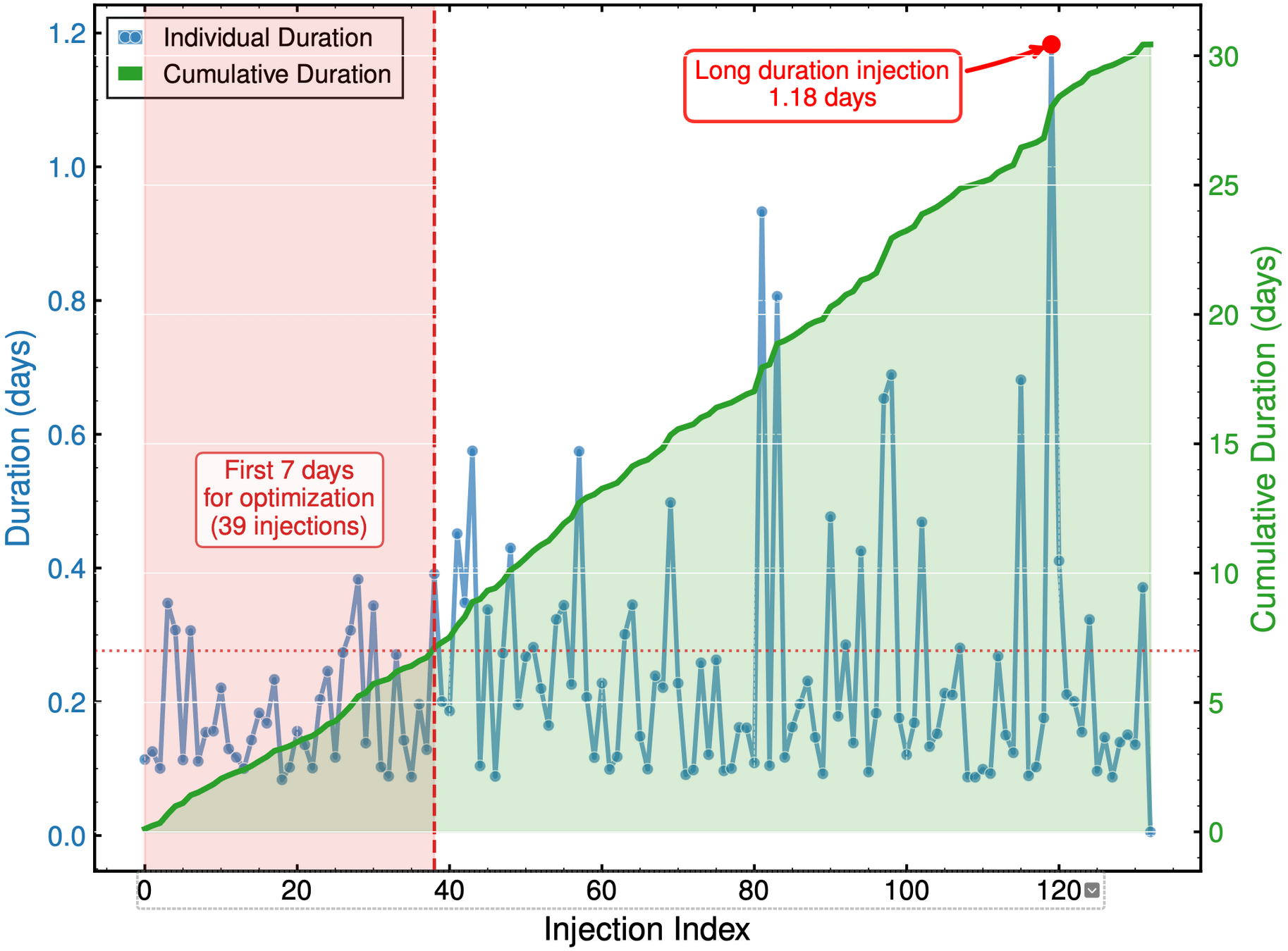
Detection statistics from our AI model showing O1 events

HW et al 2024 MLST 5 015046

GW151226

GW151012

LVK. PRD (2016). arXiv:1602.03839

Sci4MLGW@ICERM (June 2025)

GW Search & Parameter Estimation Challenges with AI Models:

Convincing the scientific community of the pipeline's validity and the statistical significance of new discoveries remains difficult despite the model's ability to identify potential gravitational wave signals.
In parameter estimation, AI models' lack of interpretability requires substantial additional scientific validation to ensure credibility and acceptance of results.
Results from AI models often lack robustness across different noise realizations and are difficult to calibrate against established methods.
Scientific papers using AI methods must dedicate significant space to validation procedures, comparing against traditional methods and demonstrating reliability across multiple test cases.

AAD for GW detection Guided by LLM-informed Evo-MCTS

He Wang | ICTP-AP, UCAS

Why Do We Trust Traditional Models?

Key Trust Factors:

✓ Interpretable: Parameters have physical meaning
✓ Built-in uncertainties: Input uncertainties propagate to outputs
✓ Model selection: Balance simplicity with accuracy
✓ Scientific insight: Reduces complexity, reveals principles

Traditional Physics Approach

Input

Human-Designed Algorithm

(Based on human insight)

Output

Example: Matched Filtering,
Linear Regression

Black-Box AI Approach

Input

AI Model

(Low interpretability)

Output

Examples: CNN, AlphaGo, DINGO

Key Challenge: How can we maintain the interpretability advantages of traditional models while leveraging the power of AI approaches?

Data/
Experience

hewang@ucas.ac.cn

AAD for GW detection Guided by LLM-informed Evo-MCTS

He Wang | ICTP-AP, UCAS

Bridging Trust & Performance in GW Analysis

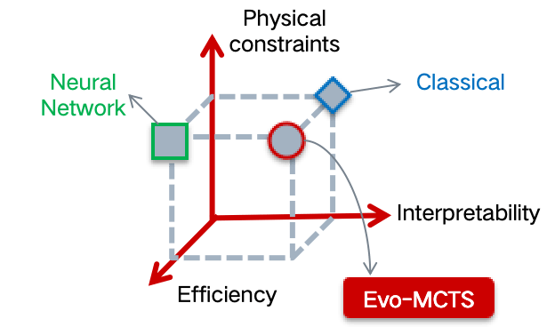
Combining the interpretability of physics with the power of AI

Our Mission: To create transparent AI systems that combine physics-based interpretability with deep learning capabilities

Interpretable AI Approach

The best of both worlds

Input

Physics-Informed
Algorithm

(High interpretability)

Output

Example: Our Approach
(Evo-MCTS)

AI Model

Physics
Knowledge

Traditional Physics Approach

Input

Human-Designed Algorithm

(Based on human insight)

Output

Example: Matched Filtering, linear regression

Black-Box AI Approach

Input

AI Model

(Low interpretability)

Output

Examples: CNN, AlphaGo, DINGO

Data/
Experience

🎯 OUR WORK

hewang@ucas.ac.cn

AAD for GW detection Guided by LLM-informed Evo-MCTS

Automated Heuristic Design: Problem Definition

He Wang | ICTP-AP, UCAS

For any complex task \(P\) (especially NP-hard problems), Automated Heuristic Design (AHD) searches for the optimal heuristic \(h^*\) within a heuristic space \(H\):

\(h^*=\underset{h \in H}{\arg \max } g(h) \)

The heuristic space \(H\) contains all feasible algorithmic solutions for task \(P\). Each heuristic \(h \in H\) maps from the set of task inputs \(I_P\) to corresponding solutions \(S_P\):

\(h: I_P \rightarrow S_P\)

Performance measure \(g(\cdot)\) evaluates each heuristic's effectiveness, \(g: H \rightarrow \mathbb{R}\). For minimization problems with objective function \(f: S_P \rightarrow \mathbb{R}\), we estimate performance by evaluating the heuristic instances \({ins}\in D \subseteq I_P\) on dataset \(D\) as follows:

\(g(h)=\mathbb{E}_{\boldsymbol{ins} \in D}[-f(h(\boldsymbol{ins}))]\)

arXiv.2410.14716

S_p

\mathbb{R}

I_p

external_knowledge
(constraint)

g(h)

HW & ZL, arXiv:2508.03661

hewang@ucas.ac.cn

AAD for GW detection Guided by LLM-informed Evo-MCTS

He Wang | ICTP-AP, UCAS

import numpy as np
import scipy.signal as signal
def pipeline_v1(strain_h1: np.ndarray, strain_l1: np.ndarray, times: np.ndarray) -> tuple[np.ndarray, np.ndarray, np.ndarray]:
    def data_conditioning(strain_h1: np.ndarray, strain_l1: np.ndarray, times: np.ndarray) -> tuple[np.ndarray, np.ndarray, np.ndarray]:
        window_length = 4096
        dt = times[1] - times[0]
        fs = 1.0 / dt
        
        def whiten_strain(strain):
            strain_zeromean = strain - np.mean(strain)
            freqs, psd = signal.welch(strain_zeromean, fs=fs, nperseg=window_length,
                                       window='hann', noverlap=window_length//2)
            smoothed_psd = np.convolve(psd, np.ones(32) / 32, mode='same')
            smoothed_psd = np.maximum(smoothed_psd, np.finfo(float).tiny)
            white_fft = np.fft.rfft(strain_zeromean) / np.sqrt(np.interp(np.fft.rfftfreq(len(strain_zeromean), d=dt), freqs, smoothed_psd))
            return np.fft.irfft(white_fft)

        whitened_h1 = whiten_strain(strain_h1)
        whitened_l1 = whiten_strain(strain_l1)
        
        return whitened_h1, whitened_l1, times
    
    def compute_metric_series(h1_data: np.ndarray, l1_data: np.ndarray, time_series: np.ndarray) -> tuple[np.ndarray, np.ndarray]:
        fs = 1 / (time_series[1] - time_series[0])
        f_h1, t_h1, Sxx_h1 = signal.spectrogram(h1_data, fs=fs, nperseg=256, noverlap=128, mode='magnitude', detrend=False)
        f_l1, t_l1, Sxx_l1 = signal.spectrogram(l1_data, fs=fs, nperseg=256, noverlap=128, mode='magnitude', detrend=False)
        tf_metric = np.mean((Sxx_h1**2 + Sxx_l1**2) / 2, axis=0)
        gps_mid_time = time_series[0] + (time_series[-1] - time_series[0]) / 2
        metric_times = gps_mid_time + (t_h1 - t_h1[-1] / 2)
        
        return tf_metric, metric_times

    def calculate_statistics(tf_metric, t_h1):
        background_level = np.median(tf_metric)
        peaks, _ = signal.find_peaks(tf_metric, height=background_level * 1.0, distance=2, prominence=background_level * 0.3)
        peak_times = t_h1[peaks]
        peak_heights = tf_metric[peaks]
        peak_deltat = np.full(len(peak_times), 10.0)  # Fixed uncertainty value
        return peak_times, peak_heights, peak_deltat

    whitened_h1, whitened_l1, data_times = data_conditioning(strain_h1, strain_l1, times)
    tf_metric, metric_times = compute_metric_series(whitened_h1, whitened_l1, data_times)
    peak_times, peak_heights, peak_deltat = calculate_statistics(tf_metric, metric_times)
    
    return peak_times, peak_heights, peak_deltat

Input: H1 and L1 detector strains, time array | Output: Event times, significance values, and time uncertainties

S_p

\mathbb{R}

I_p

external_knowledge
(constraint)

g(h)

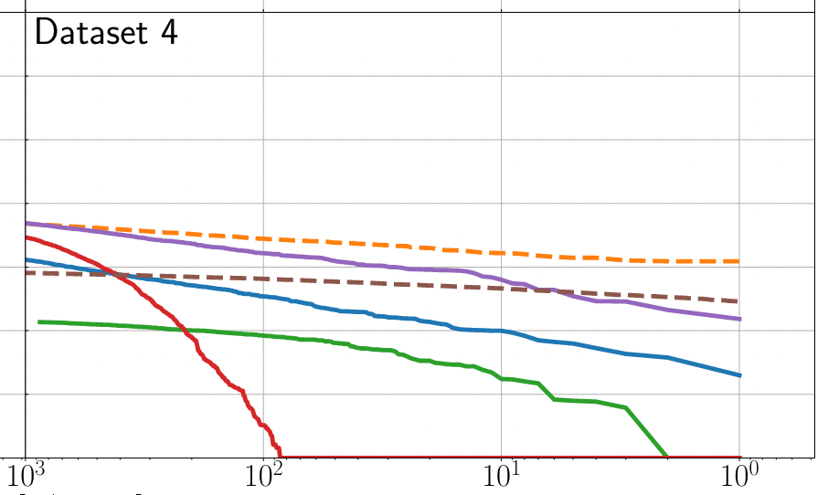
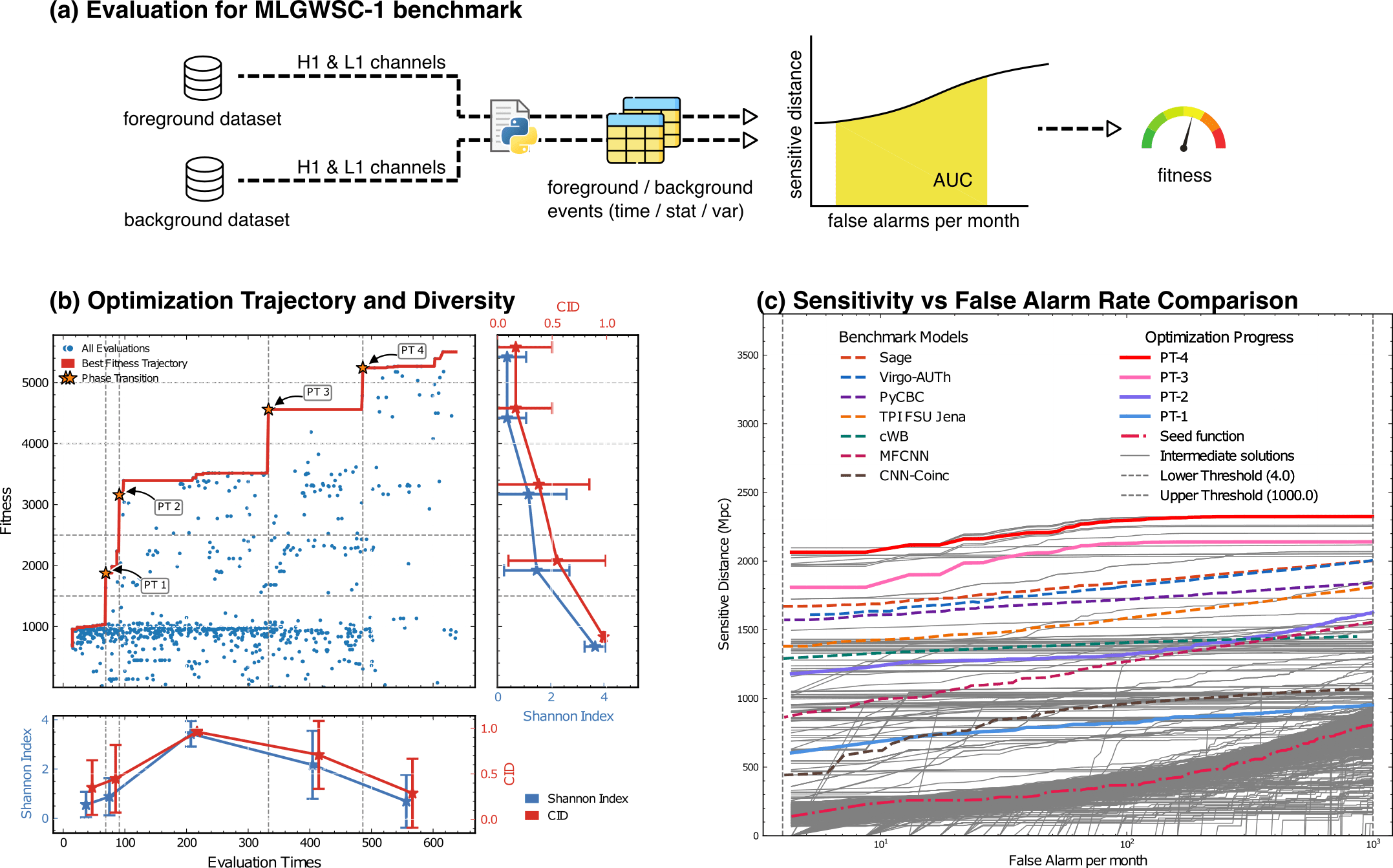
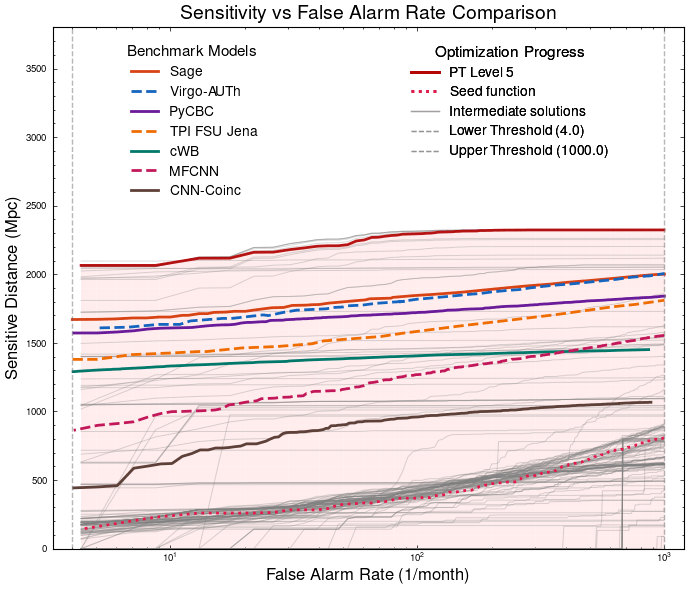
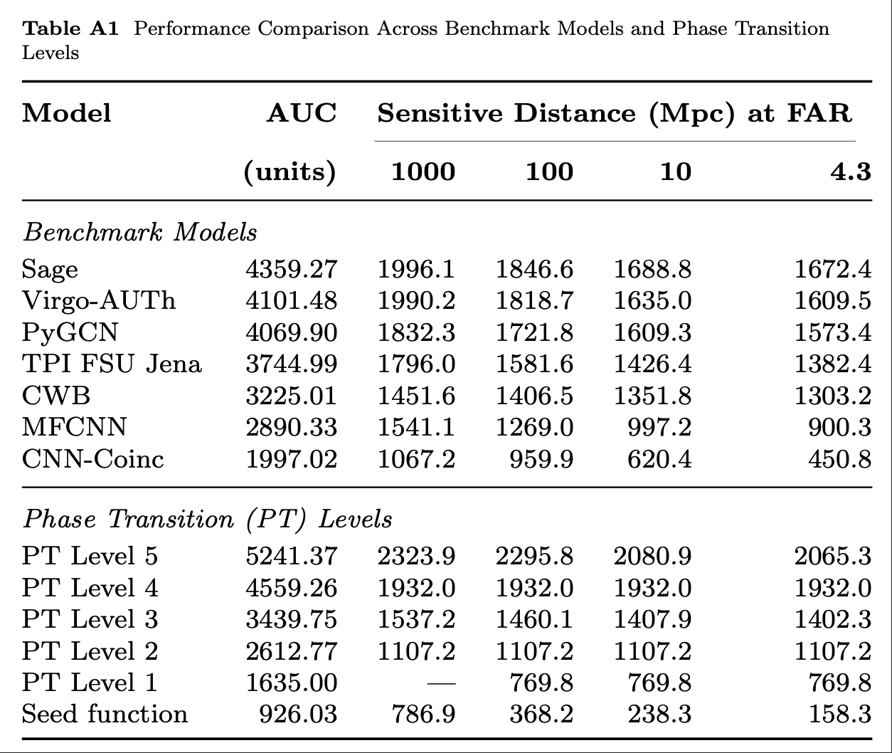
Optimization Target: Maximizing Area Under Curve (AUC) in the 1-1000Hz false alarms per-year range, balancing detection sensitivity and false alarm rates across algorithm generations

Automated Heuristic Design: Problem Definition

HW & ZL, arXiv:2508.03661

MLGWSC-1 benchmark

Problem: Pipeline Workflow

Conditions raw detector data (whitening)
Computes time-frequency metrics
Identifies peaks above background
Returns event candidates with timestamps

AAD for GW detection Guided by LLM-informed Evo-MCTS

He Wang | ICTP-AP, UCAS

Algorithmic Exploration：LLM Prompt Engineering

external_knowledge
(constraint)

g(h)

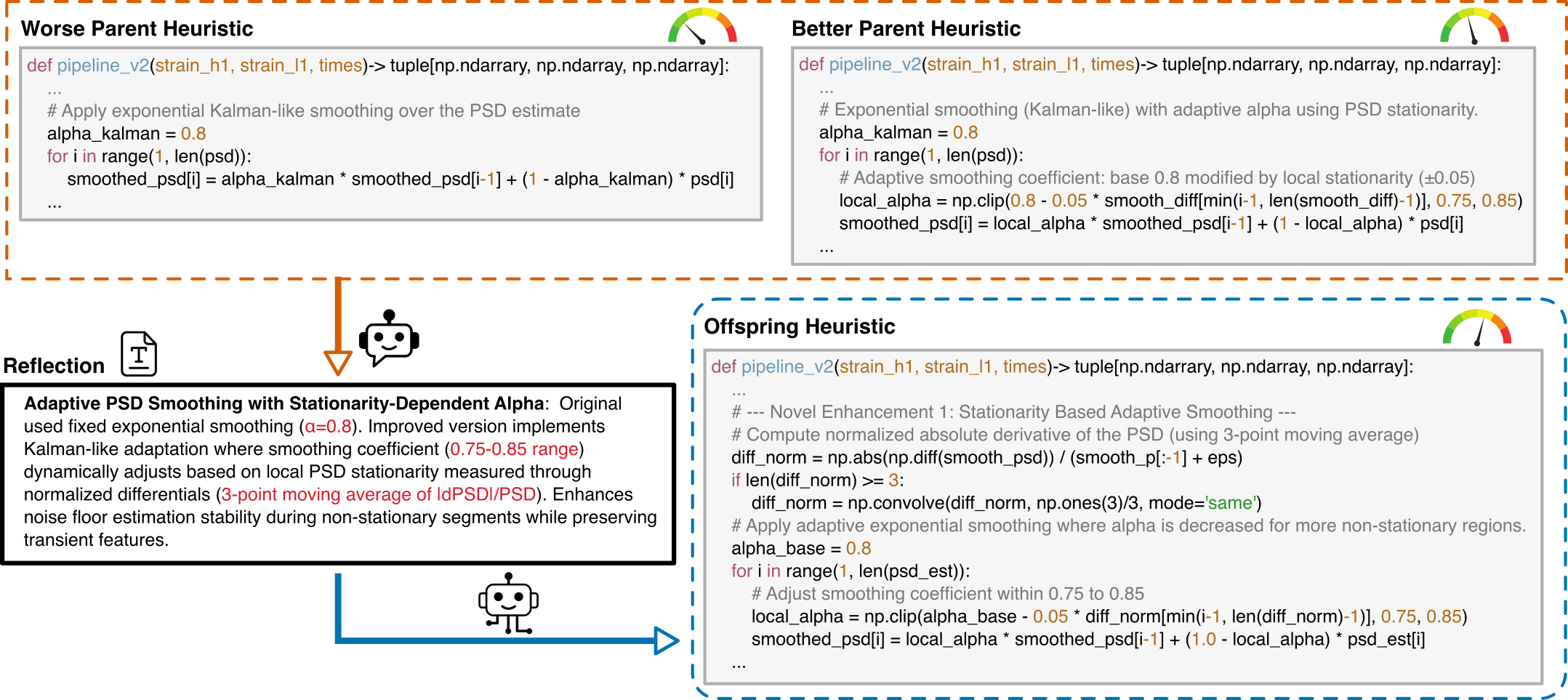
Prompt Structure for Algorithm Evolution

This template guides the LLM to generate optimized gravitational wave detection algorithms by learning from comparative examples.

Key Components:

Expert role establishment
Example pair analysis (worse/better algorithm)
Reflection on improvements
Targeted new algorithm generation
Strict output format enforcement

You are an expert in gravitational wave signal detection algorithms. Your task is to design heuristics that can effectively solve optimization problems.

{prompt_task}

I have analyzed two algorithms and provided a reflection on their differences. 

[Worse code]
{worse_code}

[Better code]
{better_code}

[Reflection]
{reflection}

Based on this reflection, please write an improved algorithm according to the reflection. 
First, describe the design idea and main steps of your algorithm in one sentence. The description must be inside a brace outside the code implementation. Next, implement it in Python as a function named '{func_name}'.
This function should accept {input_count} input(s): {joined_inputs}. The function should return {output_count} output(s): {joined_outputs}. 
{inout_inf} {other_inf}

Do not give additional explanations.

One Prompt Template for MLGWSC1 Algorithm Synthesis

hewang@ucas.ac.cn

HW & ZL, arXiv:2508.03661

AAD for GW detection Guided by LLM-informed Evo-MCTS

Algorithmic Synergy: MCTS, Evolution & LLM Agents

He Wang | ICTP-AP, UCAS

Within each evolutionary iteration, MCTS decomposes complex signal detection problems into manageable decision sequences, enabling depth-wise and path-wise exploration of algorithmic possibilities.
We propose four evolutionary operations for MCTS expansion: Parent Crossover (PC) combines information from nodes at the parent level, Sibling Crossover (SC) exchanges features between nodes sharing the same parent, Point Mutation (PM) introduces random perturbations to individual nodes, and Path-wise Crossover (PWC) synthesizes information along complete trajectories from root to leaf.

hewang@ucas.ac.cn

AAD for GW detection Guided by LLM-informed Evo-MCTS

Algorithmic Synergy: MCTS, Evolution & LLM Agents

He Wang | ICTP-AP, UCAS

hewang@ucas.ac.cn

deepseek-R1 for reflection generation
o3-mini-medium for code generation

LLM-Driven Algorithmic Evolution Through Reflective Code Synthesis.

AAD for GW detection Guided by LLM-informed Evo-MCTS

Algorithmic Synergy: MCTS, Evolution & LLM Agents

He Wang | ICTP-AP, UCAS

hewang@ucas.ac.cn

deepseek-R1 for reflection generation
o3-mini-medium for code generation

AAD for GW detection Guided by LLM-informed Evo-MCTS

Evaluation for MLGWSC-1 benchmark

LLM-Driven Algorithmic Evolution Through Reflective Code Synthesis.

LLM-Informed Evo-MCTS for AAD

MLGWSC1 Benchmark: Optimization Performance Results

He Wang | ICTP-AP, UCAS

Pipeline Workflow

Conditions raw detector data (whitening)
Computes time-frequency metrics
Identifies peaks above background
Returns event candidates with timestamps

Diversity in Evolutionary Computation

Population encoding:

Removing comments and docstrings using abstract-syntax tree,
standardizing code snippets into a common coding style (e.g., PEP81),
Convert code snippets to vector representations using a code embedding model.

hewang@ucas.ac.cn

HW & ZL, arXiv:2508.03661

AAD for GW detection Guided by LLM-informed Evo-MCTS

MLGWSC1 Benchmark: Optimization Performance Results

He Wang | ICTP-AP, UCAS

hewang@ucas.ac.cn

HW & ZL, arXiv:2508.03661

AAD for GW detection Guided by LLM-informed Evo-MCTS

Automated exploration of algorithm parameter space

Benchmarking against state-of-the-art methods

MLGWSC1 Benchmark: Optimization Performance Results

He Wang | ICTP-AP, UCAS

Refs of Benchmark Models

Sage: 2501.13846 [gr-qc]
Virgo-AUTh / TPI FSU Jena: PRD 110, 024024 (2024)
Others: PRD 107, 023021 (2023)

hewang@ucas.ac.cn

HW & ZL, arXiv:2508.03661

20.2%

23.4%

AAD for GW detection Guided by LLM-informed Evo-MCTS

MLGWSC1 Benchmark: Optimization Performance Results

He Wang | ICTP-AP, UCAS

hewang@ucas.ac.cn

HW & ZL, arXiv:2508.03661

AAD for GW detection Guided by LLM-informed Evo-MCTS

PyCBC (linear-core)

cWB (nonlinear-core)

Simple filters (non-linear)

CNN-like (highly non-linear)

Automated exploration of algorithm parameter space

Benchmarking against state-of-the-art methods

20.2%

23.4%

Interpretability Analysis

He Wang | ICTP-AP, UCAS

hewang@ucas.ac.cn

HW & ZL, arXiv:2508.03661

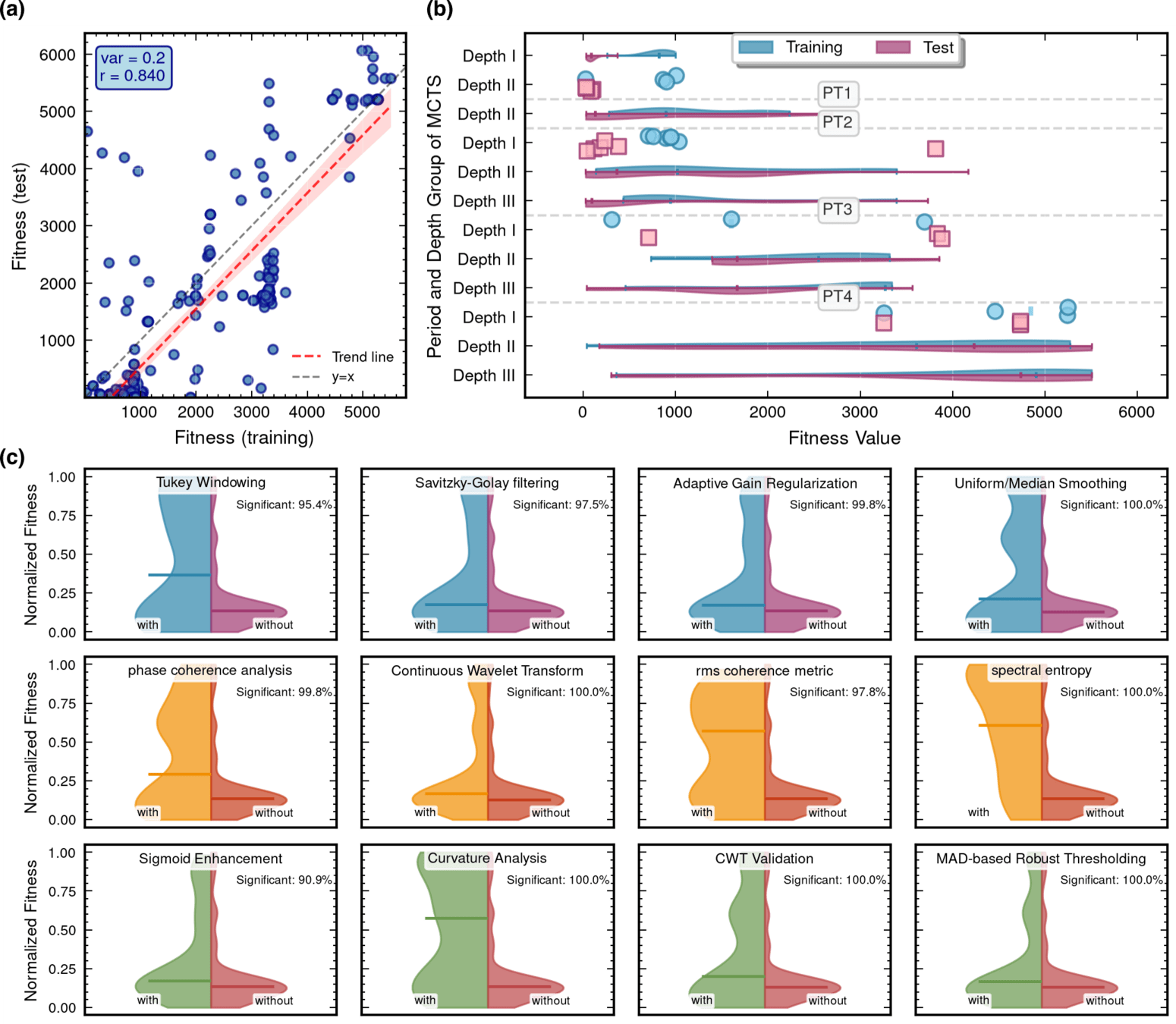
Algorithmic Component Impact Analysis.

A comprehensive technique impact analysis using controlled comparative methodology

AAD for GW detection Guided by LLM-informed Evo-MCTS

import numpy as np
import scipy.signal as signal
from scipy.signal.windows import tukey
from scipy.signal import savgol_filter

def pipeline_v2(strain_h1: np.ndarray, strain_l1: np.ndarray, times: np.ndarray) -> tuple[np.ndarray, np.ndarray, np.ndarray]:
    """
    The pipeline function processes gravitational wave data from the H1 and L1 detectors to identify potential gravitational wave signals.
    It takes strain_h1 and strain_l1 numpy arrays containing detector data, and times array with corresponding time points.
    The function returns a tuple of three numpy arrays: peak_times containing GPS times of identified events,
    peak_heights with significance values of each peak, and peak_deltat showing time window uncertainty for each peak.
    """
    eps = np.finfo(float).tiny
    dt = times[1] - times[0]
    fs = 1.0 / dt
    # Base spectrogram parameters
    base_nperseg = 256
    base_noverlap = base_nperseg // 2
    medfilt_kernel = 101       # odd kernel size for robust detrending
    uncertainty_window = 5     # half-window for local timing uncertainty

    # -------------------- Stage 1: Robust Baseline Detrending --------------------
    # Remove long-term trends using a median filter for each channel.
    detrended_h1 = strain_h1 - signal.medfilt(strain_h1, kernel_size=medfilt_kernel)
    detrended_l1 = strain_l1 - signal.medfilt(strain_l1, kernel_size=medfilt_kernel)

    # -------------------- Stage 2: Adaptive Whitening with Enhanced PSD Smoothing --------------------
    def adaptive_whitening(strain: np.ndarray) -> np.ndarray:
        # Center the signal.
        centered = strain - np.mean(strain)
        n_samples = len(centered)
        # Adaptive window length: between 5 and 30 seconds
        win_length_sec = np.clip(n_samples / fs / 20, 5, 30)
        nperseg_adapt = int(win_length_sec * fs)
        nperseg_adapt = max(10, min(nperseg_adapt, n_samples))
        
        # Create a Tukey window with 75% overlap.
        tukey_alpha = 0.25
        win = tukey(nperseg_adapt, alpha=tukey_alpha)
        noverlap_adapt = int(nperseg_adapt * 0.75)
        if noverlap_adapt >= nperseg_adapt:
            noverlap_adapt = nperseg_adapt - 1
        
        # Estimate the power spectral density (PSD) using Welch's method.
        freqs, psd = signal.welch(centered, fs=fs, nperseg=nperseg_adapt,
                                  noverlap=noverlap_adapt, window=win, detrend='constant')
        psd = np.maximum(psd, eps)
        
        # Compute relative differences for PSD stationarity measure.
        diff_arr = np.abs(np.diff(psd)) / (psd[:-1] + eps)
        # Smooth the derivative with a moving average.
        if len(diff_arr) >= 3:
            smooth_diff = np.convolve(diff_arr, np.ones(3)/3, mode='same')
        else:
            smooth_diff = diff_arr
        
        # Exponential smoothing (Kalman-like) with adaptive alpha using PSD stationarity.
        smoothed_psd = np.copy(psd)
        for i in range(1, len(psd)):
            # Adaptive smoothing coefficient: base 0.8 modified by local stationarity (±0.05)
            local_alpha = np.clip(0.8 - 0.05 * smooth_diff[min(i-1, len(smooth_diff)-1)], 0.75, 0.85)
            smoothed_psd[i] = local_alpha * smoothed_psd[i-1] + (1 - local_alpha) * psd[i]
            
        # Compute Tikhonov regularization gain based on deviation from median PSD.
        noise_baseline = np.median(smoothed_psd)
        raw_gain = (smoothed_psd / (noise_baseline + eps)) - 1.0
        
        # Compute a causal-like gradient using the Savitzky-Golay filter.
        win_len = 11 if len(smoothed_psd) >= 11 else ((len(smoothed_psd)//2)*2+1)
        polyorder = 2 if win_len > 2 else 1
        delta_freq = np.mean(np.diff(freqs))
        grad_psd = savgol_filter(smoothed_psd, win_len, polyorder, deriv=1, delta=delta_freq, mode='interp')
        
        # Nonlinear scaling via sigmoid to enhance gradient differences.
        sigmoid = lambda x: 1.0 / (1.0 + np.exp(-x))
        scaling_factor = 1.0 + 2.0 * sigmoid(np.abs(grad_psd) / (np.median(smoothed_psd) + eps))
        
        # Compute adaptive gain factors with nonlinear scaling.
        gain = 1.0 - np.exp(-0.5 * scaling_factor * raw_gain)
        gain = np.clip(gain, -8.0, 8.0)
        
        # FFT-based whitening: interpolate gain and PSD onto FFT frequency bins.
        signal_fft = np.fft.rfft(centered)
        freq_bins = np.fft.rfftfreq(n_samples, d=dt)
        interp_gain = np.interp(freq_bins, freqs, gain, left=gain[0], right=gain[-1])
        interp_psd = np.interp(freq_bins, freqs, smoothed_psd, left=smoothed_psd[0], right=smoothed_psd[-1])
        denom = np.sqrt(interp_psd) * (np.abs(interp_gain) + eps)
        denom = np.maximum(denom, eps)
        white_fft = signal_fft / denom
        whitened = np.fft.irfft(white_fft, n=n_samples)
        return whitened

    # Whiten H1 and L1 channels using the adapted method.
    white_h1 = adaptive_whitening(detrended_h1)
    white_l1 = adaptive_whitening(detrended_l1)

    # -------------------- Stage 3: Coherent Time-Frequency Metric with Frequency-Conditioned Regularization --------------------
    def compute_coherent_metric(w1: np.ndarray, w2: np.ndarray) -> tuple[np.ndarray, np.ndarray]:
        # Compute complex spectrograms preserving phase information.
        f1, t_spec, Sxx1 = signal.spectrogram(w1, fs=fs, nperseg=base_nperseg,
                                              noverlap=base_noverlap, mode='complex', detrend=False)
        f2, t_spec2, Sxx2 = signal.spectrogram(w2, fs=fs, nperseg=base_nperseg,
                                               noverlap=base_noverlap, mode='complex', detrend=False)
        # Ensure common time axis length.
        common_len = min(len(t_spec), len(t_spec2))
        t_spec = t_spec[:common_len]
        Sxx1 = Sxx1[:, :common_len]
        Sxx2 = Sxx2[:, :common_len]
        
        # Compute phase differences and coherence between detectors.
        phase_diff = np.angle(Sxx1) - np.angle(Sxx2)
        phase_coherence = np.abs(np.cos(phase_diff))
        
        # Estimate median PSD per frequency bin from the spectrograms.
        psd1 = np.median(np.abs(Sxx1)**2, axis=1)
        psd2 = np.median(np.abs(Sxx2)**2, axis=1)
        
        # Frequency-conditioned regularization gain (reflection-guided).
        lambda_f = 0.5 * ((np.median(psd1) / (psd1 + eps)) + (np.median(psd2) / (psd2 + eps)))
        lambda_f = np.clip(lambda_f, 1e-4, 1e-2)
        # Regularization denominator integrating detector PSDs and lambda.
        reg_denom = (psd1[:, None] + psd2[:, None] + lambda_f[:, None] + eps)
        
        # Weighted phase coherence that balances phase alignment with noise levels.
        weighted_comp = phase_coherence / reg_denom
        
        # Compute axial (frequency) second derivatives as curvature estimates.
        d2_coh = np.gradient(np.gradient(phase_coherence, axis=0), axis=0)
        avg_curvature = np.mean(np.abs(d2_coh), axis=0)
        
        # Nonlinear activation boost using tanh for regions of high curvature.
        nonlinear_boost = np.tanh(5 * avg_curvature)
        linear_boost = 1.0 + 0.1 * avg_curvature
        
        # Cross-detector synergy: weight derived from global median consistency.
        novel_weight = np.mean((np.median(psd1) + np.median(psd2)) / (psd1[:, None] + psd2[:, None] + eps), axis=0)
        
        # Integrated time-frequency metric combining all enhancements.
        tf_metric = np.sum(weighted_comp * linear_boost * (1.0 + nonlinear_boost), axis=0) * novel_weight
        
        # Adjust the spectrogram time axis to account for window delay.
        metric_times = t_spec + times[0] + (base_nperseg / 2) / fs
        return tf_metric, metric_times

    tf_metric, metric_times = compute_coherent_metric(white_h1, white_l1)

    # -------------------- Stage 4: Multi-Resolution Thresholding with Octave-Spaced Dyadic Wavelet Validation --------------------
    def multi_resolution_thresholding(metric: np.ndarray, times_arr: np.ndarray) -> tuple[np.ndarray, np.ndarray, np.ndarray]:
        # Robust background estimation with median and MAD.
        bg_level = np.median(metric)
        mad_val = np.median(np.abs(metric - bg_level))
        robust_std = 1.4826 * mad_val
        threshold = bg_level + 1.5 * robust_std

        # Identify candidate peaks using prominence and minimum distance criteria.
        peaks, _ = signal.find_peaks(metric, height=threshold, distance=2, prominence=0.8 * robust_std)
        if peaks.size == 0:
            return np.array([]), np.array([]), np.array([])

        # Local uncertainty estimation using a Gaussian-weighted convolution.
        win_range = np.arange(-uncertainty_window, uncertainty_window + 1)
        sigma = uncertainty_window / 2.5
        gauss_kernel = np.exp(-0.5 * (win_range / sigma) ** 2)
        gauss_kernel /= np.sum(gauss_kernel)
        weighted_mean = np.convolve(metric, gauss_kernel, mode='same')
        weighted_sq = np.convolve(metric ** 2, gauss_kernel, mode='same')
        variances = np.maximum(weighted_sq - weighted_mean ** 2, 0.0)
        uncertainties = np.sqrt(variances)
        uncertainties = np.maximum(uncertainties, 0.01)

        valid_times = []
        valid_heights = []
        valid_uncerts = []
        n_metric = len(metric)

        # Compute a simple second derivative for local curvature checking.
        if n_metric > 2:
            second_deriv = np.diff(metric, n=2)
            second_deriv = np.pad(second_deriv, (1, 1), mode='edge')
        else:
            second_deriv = np.zeros_like(metric)

        # Use octave-spaced scales (dyadic wavelet validation) to validate peak significance.
        widths = np.arange(1, 9)  # approximate scales 1 to 8
        for peak in peaks:
            # Skip peaks lacking sufficient negative curvature.
            if second_deriv[peak] > -0.1 * robust_std:
                continue
            local_start = max(0, peak - uncertainty_window)
            local_end = min(n_metric, peak + uncertainty_window + 1)
            local_segment = metric[local_start:local_end]
            if len(local_segment) < 3:
                continue
            try:
                cwt_coeff = signal.cwt(local_segment, signal.ricker, widths)
            except Exception:
                continue
            max_coeff = np.max(np.abs(cwt_coeff))
            # Threshold for validating the candidate using local MAD.
            cwt_thresh = mad_val * np.sqrt(2 * np.log(len(local_segment) + eps))
            if max_coeff >= cwt_thresh:
                valid_times.append(times_arr[peak])
                valid_heights.append(metric[peak])
                valid_uncerts.append(uncertainties[peak])

        if len(valid_times) == 0:
            return np.array([]), np.array([]), np.array([])
        return np.array(valid_times), np.array(valid_heights), np.array(valid_uncerts)

    peak_times, peak_heights, peak_deltat = multi_resolution_thresholding(tf_metric, metric_times)
    return peak_times, peak_heights, peak_deltat

Automatically discover and interpret the value of nonlinear algorithms
Facilitating new knowledge production along with experience guidance

PT Level 5

Interpretability Analysis: PT Level 5

He Wang | ICTP-AP, UCAS

import numpy as np
import scipy.signal as signal
from scipy.signal.windows import tukey
from scipy.signal import savgol_filter

def pipeline_v2(strain_h1: np.ndarray, strain_l1: np.ndarray, times: np.ndarray) -> tuple[np.ndarray, np.ndarray, np.ndarray]:
    """
    The pipeline function processes gravitational wave data from the H1 and L1 detectors to identify potential gravitational wave signals.
    It takes strain_h1 and strain_l1 numpy arrays containing detector data, and times array with corresponding time points.
    The function returns a tuple of three numpy arrays: peak_times containing GPS times of identified events,
    peak_heights with significance values of each peak, and peak_deltat showing time window uncertainty for each peak.
    """
    eps = np.finfo(float).tiny
    dt = times[1] - times[0]
    fs = 1.0 / dt
    # Base spectrogram parameters
    base_nperseg = 256
    base_noverlap = base_nperseg // 2
    medfilt_kernel = 101       # odd kernel size for robust detrending
    uncertainty_window = 5     # half-window for local timing uncertainty

    # -------------------- Stage 1: Robust Baseline Detrending --------------------
    # Remove long-term trends using a median filter for each channel.
    detrended_h1 = strain_h1 - signal.medfilt(strain_h1, kernel_size=medfilt_kernel)
    detrended_l1 = strain_l1 - signal.medfilt(strain_l1, kernel_size=medfilt_kernel)

    # -------------------- Stage 2: Adaptive Whitening with Enhanced PSD Smoothing --------------------
    def adaptive_whitening(strain: np.ndarray) -> np.ndarray:
        # Center the signal.
        centered = strain - np.mean(strain)
        n_samples = len(centered)
        # Adaptive window length: between 5 and 30 seconds
        win_length_sec = np.clip(n_samples / fs / 20, 5, 30)
        nperseg_adapt = int(win_length_sec * fs)
        nperseg_adapt = max(10, min(nperseg_adapt, n_samples))
        
        # Create a Tukey window with 75% overlap.
        tukey_alpha = 0.25
        win = tukey(nperseg_adapt, alpha=tukey_alpha)
        noverlap_adapt = int(nperseg_adapt * 0.75)
        if noverlap_adapt >= nperseg_adapt:
            noverlap_adapt = nperseg_adapt - 1
        
        # Estimate the power spectral density (PSD) using Welch's method.
        freqs, psd = signal.welch(centered, fs=fs, nperseg=nperseg_adapt,
                                  noverlap=noverlap_adapt, window=win, detrend='constant')
        psd = np.maximum(psd, eps)
        
        # Compute relative differences for PSD stationarity measure.
        diff_arr = np.abs(np.diff(psd)) / (psd[:-1] + eps)
        # Smooth the derivative with a moving average.
        if len(diff_arr) >= 3:
            smooth_diff = np.convolve(diff_arr, np.ones(3)/3, mode='same')
        else:
            smooth_diff = diff_arr
        
        # Exponential smoothing (Kalman-like) with adaptive alpha using PSD stationarity.
        smoothed_psd = np.copy(psd)
        for i in range(1, len(psd)):
            # Adaptive smoothing coefficient: base 0.8 modified by local stationarity (±0.05)
            local_alpha = np.clip(0.8 - 0.05 * smooth_diff[min(i-1, len(smooth_diff)-1)], 0.75, 0.85)
            smoothed_psd[i] = local_alpha * smoothed_psd[i-1] + (1 - local_alpha) * psd[i]
            
        # Compute Tikhonov regularization gain based on deviation from median PSD.
        noise_baseline = np.median(smoothed_psd)
        raw_gain = (smoothed_psd / (noise_baseline + eps)) - 1.0
        
        # Compute a causal-like gradient using the Savitzky-Golay filter.
        win_len = 11 if len(smoothed_psd) >= 11 else ((len(smoothed_psd)//2)*2+1)
        polyorder = 2 if win_len > 2 else 1
        delta_freq = np.mean(np.diff(freqs))
        grad_psd = savgol_filter(smoothed_psd, win_len, polyorder, deriv=1, delta=delta_freq, mode='interp')
        
        # Nonlinear scaling via sigmoid to enhance gradient differences.
        sigmoid = lambda x: 1.0 / (1.0 + np.exp(-x))
        scaling_factor = 1.0 + 2.0 * sigmoid(np.abs(grad_psd) / (np.median(smoothed_psd) + eps))
        
        # Compute adaptive gain factors with nonlinear scaling.
        gain = 1.0 - np.exp(-0.5 * scaling_factor * raw_gain)
        gain = np.clip(gain, -8.0, 8.0)
        
        # FFT-based whitening: interpolate gain and PSD onto FFT frequency bins.
        signal_fft = np.fft.rfft(centered)
        freq_bins = np.fft.rfftfreq(n_samples, d=dt)
        interp_gain = np.interp(freq_bins, freqs, gain, left=gain[0], right=gain[-1])
        interp_psd = np.interp(freq_bins, freqs, smoothed_psd, left=smoothed_psd[0], right=smoothed_psd[-1])
        denom = np.sqrt(interp_psd) * (np.abs(interp_gain) + eps)
        denom = np.maximum(denom, eps)
        white_fft = signal_fft / denom
        whitened = np.fft.irfft(white_fft, n=n_samples)
        return whitened

    # Whiten H1 and L1 channels using the adapted method.
    white_h1 = adaptive_whitening(detrended_h1)
    white_l1 = adaptive_whitening(detrended_l1)

    # -------------------- Stage 3: Coherent Time-Frequency Metric with Frequency-Conditioned Regularization --------------------
    def compute_coherent_metric(w1: np.ndarray, w2: np.ndarray) -> tuple[np.ndarray, np.ndarray]:
        # Compute complex spectrograms preserving phase information.
        f1, t_spec, Sxx1 = signal.spectrogram(w1, fs=fs, nperseg=base_nperseg,
                                              noverlap=base_noverlap, mode='complex', detrend=False)
        f2, t_spec2, Sxx2 = signal.spectrogram(w2, fs=fs, nperseg=base_nperseg,
                                               noverlap=base_noverlap, mode='complex', detrend=False)
        # Ensure common time axis length.
        common_len = min(len(t_spec), len(t_spec2))
        t_spec = t_spec[:common_len]
        Sxx1 = Sxx1[:, :common_len]
        Sxx2 = Sxx2[:, :common_len]
        
        # Compute phase differences and coherence between detectors.
        phase_diff = np.angle(Sxx1) - np.angle(Sxx2)
        phase_coherence = np.abs(np.cos(phase_diff))
        
        # Estimate median PSD per frequency bin from the spectrograms.
        psd1 = np.median(np.abs(Sxx1)**2, axis=1)
        psd2 = np.median(np.abs(Sxx2)**2, axis=1)
        
        # Frequency-conditioned regularization gain (reflection-guided).
        lambda_f = 0.5 * ((np.median(psd1) / (psd1 + eps)) + (np.median(psd2) / (psd2 + eps)))
        lambda_f = np.clip(lambda_f, 1e-4, 1e-2)
        # Regularization denominator integrating detector PSDs and lambda.
        reg_denom = (psd1[:, None] + psd2[:, None] + lambda_f[:, None] + eps)
        
        # Weighted phase coherence that balances phase alignment with noise levels.
        weighted_comp = phase_coherence / reg_denom
        
        # Compute axial (frequency) second derivatives as curvature estimates.
        d2_coh = np.gradient(np.gradient(phase_coherence, axis=0), axis=0)
        avg_curvature = np.mean(np.abs(d2_coh), axis=0)
        
        # Nonlinear activation boost using tanh for regions of high curvature.
        nonlinear_boost = np.tanh(5 * avg_curvature)
        linear_boost = 1.0 + 0.1 * avg_curvature
        
        # Cross-detector synergy: weight derived from global median consistency.
        novel_weight = np.mean((np.median(psd1) + np.median(psd2)) / (psd1[:, None] + psd2[:, None] + eps), axis=0)
        
        # Integrated time-frequency metric combining all enhancements.
        tf_metric = np.sum(weighted_comp * linear_boost * (1.0 + nonlinear_boost), axis=0) * novel_weight
        
        # Adjust the spectrogram time axis to account for window delay.
        metric_times = t_spec + times[0] + (base_nperseg / 2) / fs
        return tf_metric, metric_times

    tf_metric, metric_times = compute_coherent_metric(white_h1, white_l1)

    # -------------------- Stage 4: Multi-Resolution Thresholding with Octave-Spaced Dyadic Wavelet Validation --------------------
    def multi_resolution_thresholding(metric: np.ndarray, times_arr: np.ndarray) -> tuple[np.ndarray, np.ndarray, np.ndarray]:
        # Robust background estimation with median and MAD.
        bg_level = np.median(metric)
        mad_val = np.median(np.abs(metric - bg_level))
        robust_std = 1.4826 * mad_val
        threshold = bg_level + 1.5 * robust_std

        # Identify candidate peaks using prominence and minimum distance criteria.
        peaks, _ = signal.find_peaks(metric, height=threshold, distance=2, prominence=0.8 * robust_std)
        if peaks.size == 0:
            return np.array([]), np.array([]), np.array([])

        # Local uncertainty estimation using a Gaussian-weighted convolution.
        win_range = np.arange(-uncertainty_window, uncertainty_window + 1)
        sigma = uncertainty_window / 2.5
        gauss_kernel = np.exp(-0.5 * (win_range / sigma) ** 2)
        gauss_kernel /= np.sum(gauss_kernel)
        weighted_mean = np.convolve(metric, gauss_kernel, mode='same')
        weighted_sq = np.convolve(metric ** 2, gauss_kernel, mode='same')
        variances = np.maximum(weighted_sq - weighted_mean ** 2, 0.0)
        uncertainties = np.sqrt(variances)
        uncertainties = np.maximum(uncertainties, 0.01)

        valid_times = []
        valid_heights = []
        valid_uncerts = []
        n_metric = len(metric)

        # Compute a simple second derivative for local curvature checking.
        if n_metric > 2:
            second_deriv = np.diff(metric, n=2)
            second_deriv = np.pad(second_deriv, (1, 1), mode='edge')
        else:
            second_deriv = np.zeros_like(metric)

        # Use octave-spaced scales (dyadic wavelet validation) to validate peak significance.
        widths = np.arange(1, 9)  # approximate scales 1 to 8
        for peak in peaks:
            # Skip peaks lacking sufficient negative curvature.
            if second_deriv[peak] > -0.1 * robust_std:
                continue
            local_start = max(0, peak - uncertainty_window)
            local_end = min(n_metric, peak + uncertainty_window + 1)
            local_segment = metric[local_start:local_end]
            if len(local_segment) < 3:
                continue
            try:
                cwt_coeff = signal.cwt(local_segment, signal.ricker, widths)
            except Exception:
                continue
            max_coeff = np.max(np.abs(cwt_coeff))
            # Threshold for validating the candidate using local MAD.
            cwt_thresh = mad_val * np.sqrt(2 * np.log(len(local_segment) + eps))
            if max_coeff >= cwt_thresh:
                valid_times.append(times_arr[peak])
                valid_heights.append(metric[peak])
                valid_uncerts.append(uncertainties[peak])

        if len(valid_times) == 0:
            return np.array([]), np.array([]), np.array([])
        return np.array(valid_times), np.array(valid_heights), np.array(valid_uncerts)

    peak_times, peak_heights, peak_deltat = multi_resolution_thresholding(tf_metric, metric_times)
    return peak_times, peak_heights, peak_deltat

hewang@ucas.ac.cn

HW & ZL, arXiv:2508.03661

AAD for GW detection Guided by LLM-informed Evo-MCTS

Interpretability Analysis

He Wang | ICTP-AP, UCAS

Out-of-distribution (OOD) detection

Generalization capability and robustness of the optimized algorithms

hewang@ucas.ac.cn

HW & ZL, arXiv:2508.03661

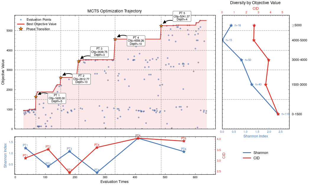
MCTS Depth-Stratified Performance Analysis.

Analyzed the relationship between MCTS tree depth and algorithm fitness across different optimization phases. The 10-layer MCTS structure was stratified into three depth groups: Depth I (depths 1-4), Depth II (depths 5-7), and Depth III (depths 8-10), representing shallow, intermediate, and deep exploration levels, respectively.

Algorithmic Component Impact Analysis.

A comprehensive technique impact analysis using controlled comparative methodology

AAD for GW detection Guided by LLM-informed Evo-MCTS

Interpretability Analysis

He Wang | ICTP-AP, UCAS

hewang@ucas.ac.cn

HW & ZL, arXiv:2508.03661

Algorithmic Component Impact Analysis.

A comprehensive technique impact analysis using controlled comparative methodology

Please analyze the following Python code snippet for gravitational wave detection and
extract technical features in JSON format.

The code typically has three main stages:
1. Data Conditioning: preprocessing, filtering, whitening, etc.
2. Time-Frequency Analysis: spectrograms, FFT, wavelets, etc.
3. Trigger Analysis: peak detection, thresholding, validation, etc.

For each stage present in the code, extract:
- Technical methods used
- Libraries and functions called
- Algorithm complexity features
- Key parameters

Code to analyze:
```python
{code_snippet}
```

Please return a JSON object with this structure:
{
  "algorithm_id": "{algorithm_id}",
  "stages": {
    "data_conditioning": {
      "present": true/false,
      "techniques": ["technique1", "technique2"],
      "libraries": ["lib1", "lib2"],
      "functions": ["func1", "func2"],
      "parameters": {"param1": "value1"},
      "complexity": "low/medium/high"
    },
    "time_frequency_analysis": {...},
    "trigger_analysis": {...}
  },
  "overall_complexity": "low/medium/high",
  "total_lines": 0,
  "unique_libraries": ["lib1", "lib2"],
  "code_quality_score": 0.0
}

Only return the JSON object, no additional text.

AAD for GW detection Guided by LLM-informed Evo-MCTS

Interpretability Analysis

He Wang | ICTP-AP, UCAS

hewang@ucas.ac.cn

HW & ZL, arXiv:2508.03661

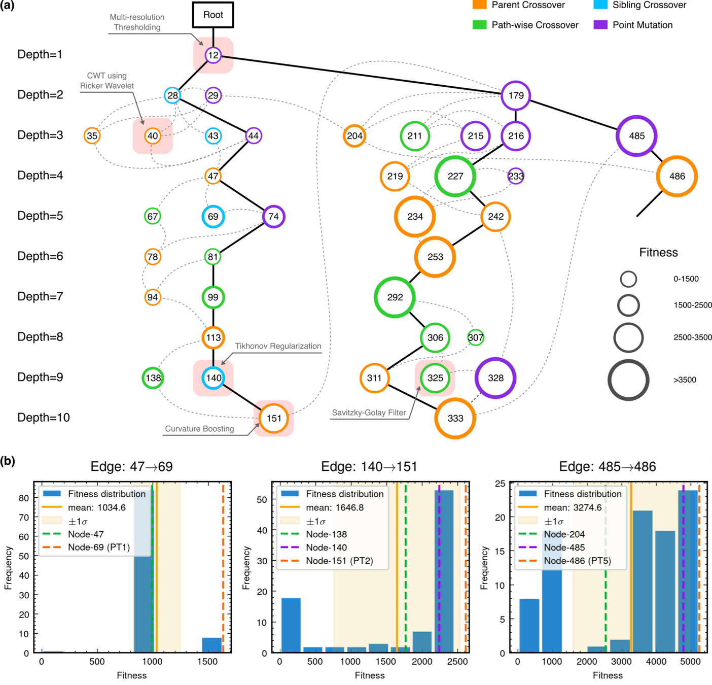
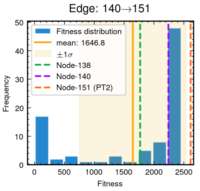
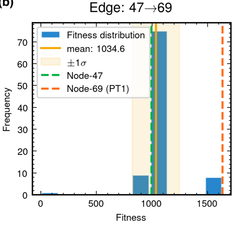
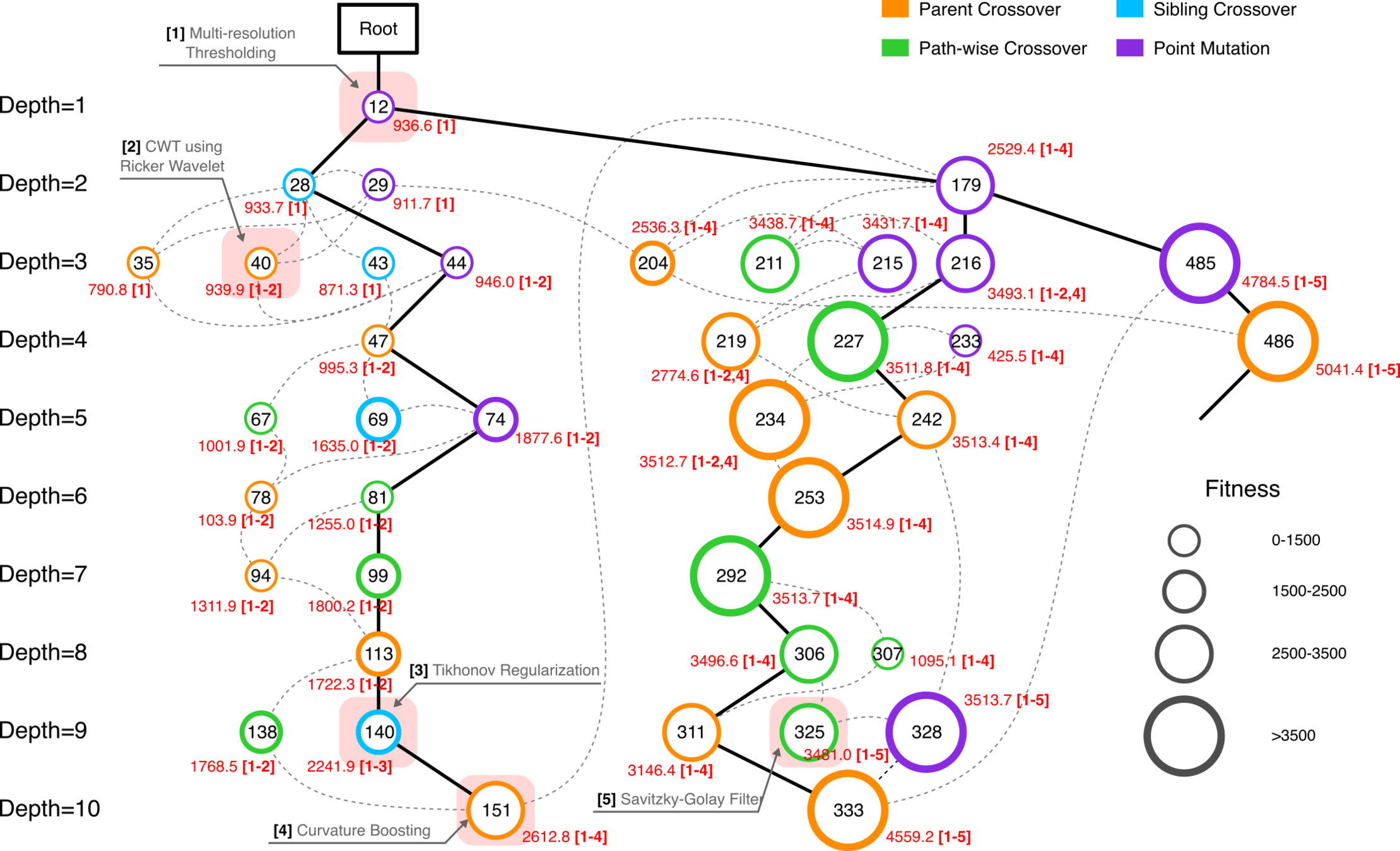
MCTS Algorithmic Evolution Pathway

Complete MCTS tree structure showing all nodes associated with the optimal algorithm.

AAD for GW detection Guided by LLM-informed Evo-MCTS

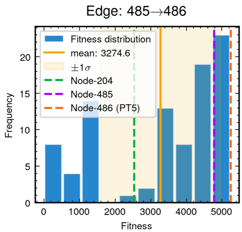
Edge robustness analysis for three critical evolutionary transitions.

Confirming the consistent discovery

Interpretability Analysis

He Wang | ICTP-AP, UCAS

hewang@ucas.ac.cn

HW & ZL, arXiv:2508.03661

Edge robustness analysis for three critical evolutionary transitions.

The distributions demonstrate the stochastic nature of LLM-driven code generation while confirming the consistent discovery of high-performance algorithmic variants.

AAD for GW detection Guided by LLM-informed Evo-MCTS

Interpretability Analysis

He Wang | ICTP-AP, UCAS

MCTS Algorithmic Evolution Pathway

Complete MCTS tree structure showing all nodes associated with the optimal algorithm (node 486, fitness=5041.4).

hewang@ucas.ac.cn

HW & ZL, arXiv:2508.03661

AAD for GW detection Guided by LLM-informed Evo-MCTS

Framework Mechanism Analysis

He Wang | ICTP-AP, UCAS

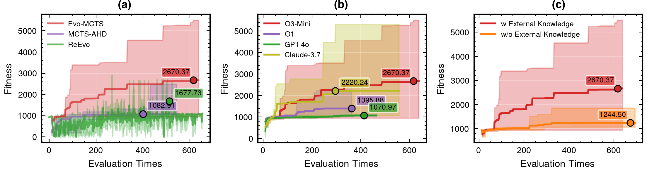
Integrated Architecture Validation

A comprehensive comparison of our integrated
Evo-MCTS framework against its constituent components operating in isolation.
- Evo-MCTS: MCTS + Self-evolve + Reflection mech.
- MCTS-AHD: MCTS framework for CO.
- ReEvo: evolutionary framework for CO.

Contributions of knowledge synthesis

Compare to w/o external knowledge
- non-linear vs linear only

hewang@ucas.ac.cn

LLM Model Selection and Robustness Analysis

Ablation study of various LLM contributions (code generator) and their robustness.
- ```
o3-mini-medium
o1-2024-12-17
gpt-4o-2024-11-20
```
```
claude-3-7-sonnet-20250219-thinking
```

HW & ZL, arXiv:2508.03661

59.1%

AAD for GW detection Guided by LLM-informed Evo-MCTS

115%

Framework Mechanism Analysis

He Wang | ICTP-AP, UCAS

Integrated Architecture Validation

A comprehensive comparison of our integrated
Evo-MCTS framework against its constituent components operating in isolation.
- Evo-MCTS: MCTS + Self-evolve + Reflection mech.
- MCTS-AHD: MCTS framework for CO.
- ReEvo: evolutionary framework for CO.

Contributions of knowledge synthesis

Compare to w/o external knowledge
- non-linear vs linear only

hewang@ucas.ac.cn

HW & ZL, arXiv:2508.03661

59.1%

AAD for GW detection Guided by LLM-informed Evo-MCTS

### External Knowledge Integration
1. **Non-linear** Processing Core Concepts:
    - Signal Transformation: 
        * Non-linear vs linear decomposition
        * Adaptive threshold mechanisms
        * Multi-scale analysis
    
    - Feature Extraction:
        * Phase space reconstruction
        * Topological data analysis
        * Wavelet-based detection
    
    - Statistical Analysis:
        * Robust estimators
        * Non-Gaussian processes
        * Higher-order statistics

2. Implementation Principles:
    - Prioritize adaptive over fixed parameters
    - Consider local vs global characteristics
    - Balance computational cost with accuracy

115%

He Wang | ICTP-AP, UCAS

hewang@ucas.ac.cn

Key Takeaways

AAD for GW detection Guided by LLM-informed Evo-MCTS

Interpretable AI Approach

The best of both worlds

Input

Physics-Informed
Algorithm

(High interpretability)

Output

Example: Our Approach
(Evo-MCTS)

AI Model

Physics
Knowledge

Traditional Physics Approach

Input

Human-Designed Algorithm

(Based on human insight)

Output

Example: Matched Filtering,
linear regression

Black-Box AI Approach

Input

AI Model

(Low interpretability)

Output

Examples: CNN, AlphaFold

Data/
Experience

🎯 OUR WORK

He Wang | ICTP-AP, UCAS

hewang@ucas.ac.cn

Key Takeaways

Any algorithm's design problem can be viewed as an optimization challenge

Numerous intermediate processes in scientific data processing, like noise modeling and experimental design, can be classified as "algorithm optimization" problems
Several analytical modeling techniques and "symbolic regression" methods in theoretical physics and cosmology can similarly be considered "algorithm optimization" issues

AAD for GW detection Guided by LLM-informed Evo-MCTS

He Wang | ICTP-AP, UCAS

hewang@ucas.ac.cn

for _ in range(num_of_audiences):
    print('Thank you for your attention! 🙏')

Acknowledgment:

AAD for GW detection Guided by LLM-informed Evo-MCTS

Key Takeaways

Interpretable AI Approach

The best of both worlds

Input

Physics-Informed
Algorithm

(High interpretability)

Output

Example: Our Approach
(Evo-MCTS)

AI Model

Physics
Knowledge

Traditional Physics Approach

Input

Human-Designed Algorithm

(Based on human insight)

Output

Example: Matched Filtering,
linear regression

Black-Box AI Approach

Input

AI Model

(Low interpretability)

Output

Examples: CNN, AlphaFold

Data/
Experience

🎯 OUR WORK

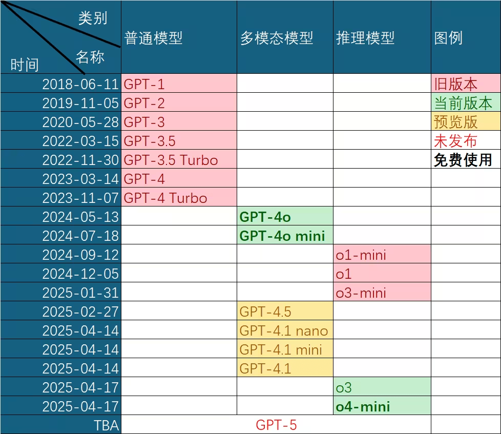
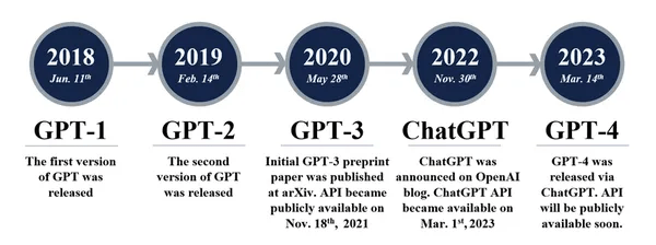
This slide: https://slides.com/iphysresearch/2025oct_natureconf

The Rise of LLMs: How Code Training Transformed AI Capabilities

Evolution of GPT Capabilities

A careful examination of GPT-3.5's capabilities reveals the origins of its emergent abilities:

Original GPT-3 gained generative abilities, world knowledge, and in-context learning through pretraining
Instruction-tuned models developed the ability to follow directions and generalize to unseen tasks
Code-trained models (code-davinci-002) acquired code comprehension
The ability to perform complex reasoning likely emerged as a byproduct of code training

GPT-3.5 series [Source: University of Edinburgh, Allen Institute for AI]

He Wang | ICTP-AP, UCAS

GPT-3 (2020)

ChatGPT (2022)

Magic: Code + Text

Interpretable Gravitational Wave Data Analysis with DL and LLMs

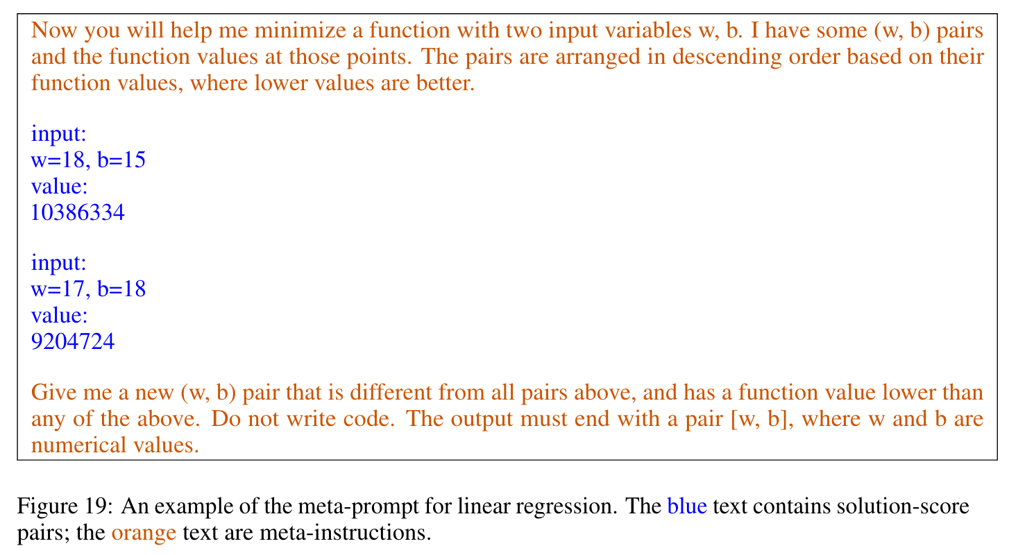
Recent research demonstrates that LLMs can solve complex optimization problems through carefully engineered prompts. DeepMind's OPRO (Optimization by PROmpting) approach showcases how LLMs can generate increasingly refined solutions through iterative prompting techniques.

OPRO: Optimization by PROmpting

Example: Least squares optimization through prompt engineering

arXiv:2309.03409 [cs.NE]

Two Directions of LLM-based Optimization

arXiv:2405.10098 [cs.NE]

He Wang | ICTP-AP, UCAS

The Optimization Potential of Large Language Models

LLMs can generate high-quality solutions to optimization problems without specialized training

Interpretable Gravitational Wave Data Analysis with DL and LLMs

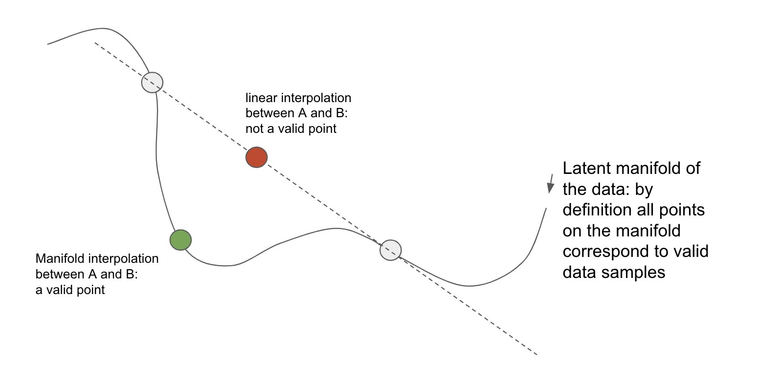
Theoretical Understanding of LLMs' Emergent Abilities

The Interpolation Theory

LLMs' ability to generate novel responses from few examples is increasingly understood as manifold interpolation rather than mere memorization:

LLMs learn a continuous semantic manifold of language during pre-training
Few-shot examples serve as anchor points in this high-dimensional space
The model interpolates between examples to generate responses for novel inputs
This enables coherent generalization beyond the training distribution
The quality of interpolation improves with model scale and training data breadth

The theory suggests that in-context learning is not "learning" in the traditional sense, but rather a form of implicit conditioning on the manifold of learned representations.

Representation Space Interpolation

He Wang | ICTP-AP, UCAS

Interpretable Gravitational Wave Data Analysis with DL and LLMs

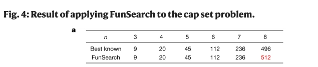
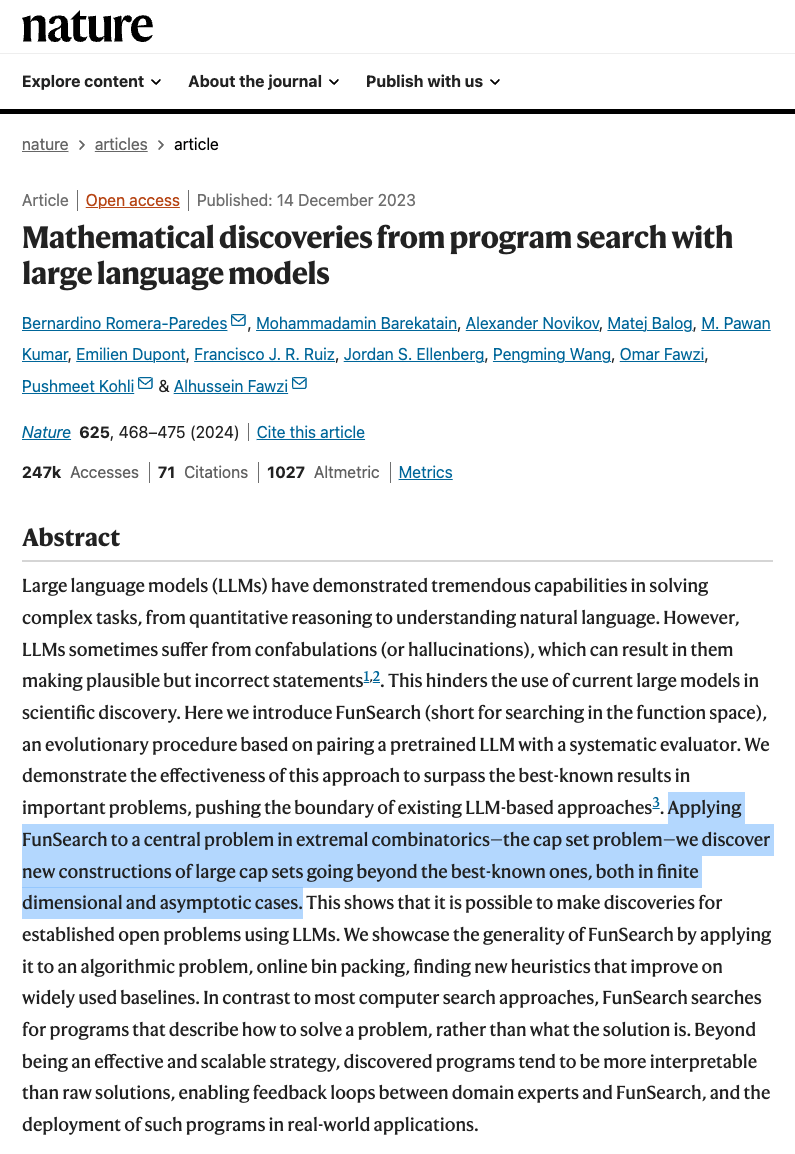
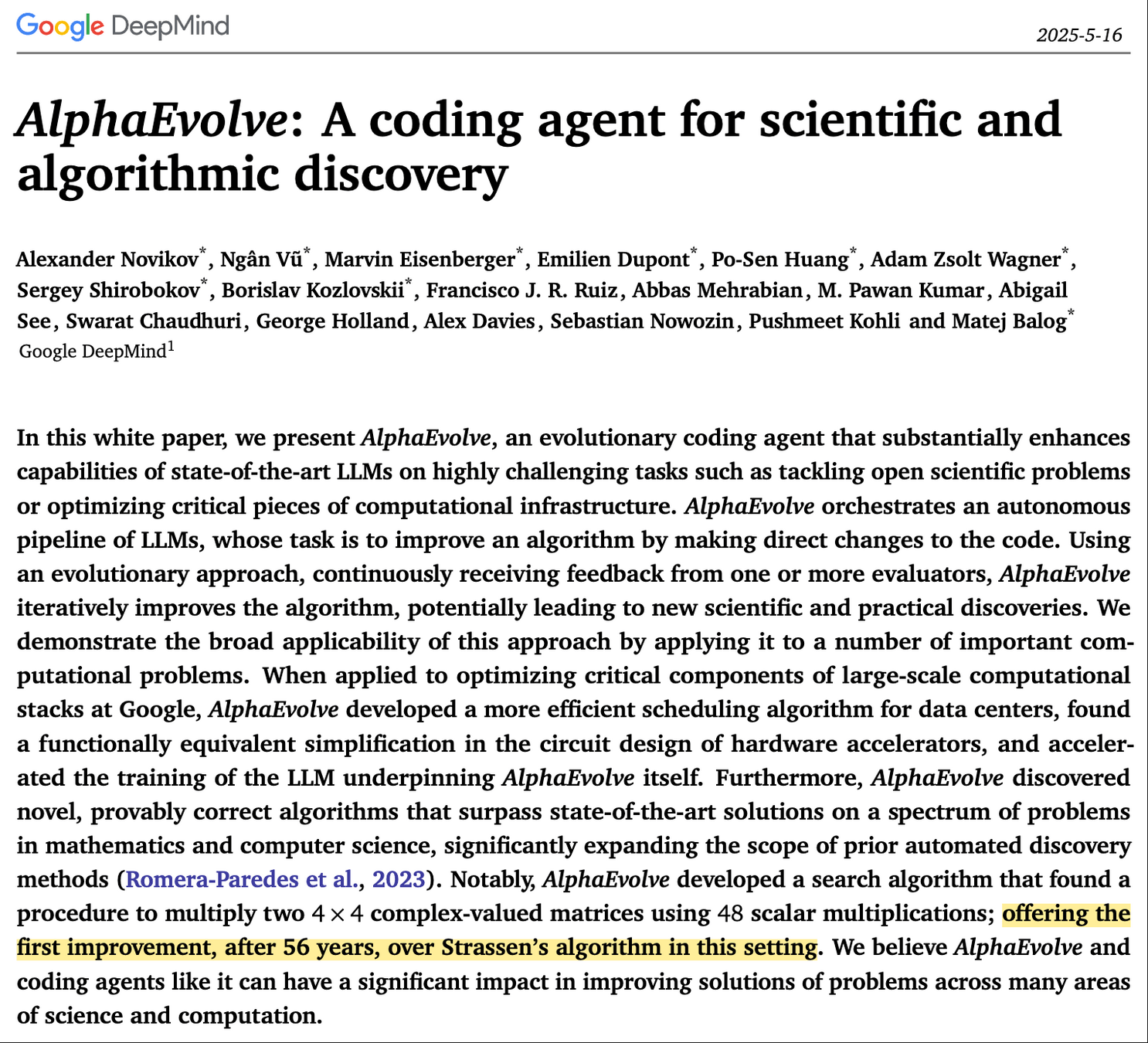
Theoretical Understanding of LLMs' Emergent Abilities

Real-world Case: FunSearch (Nature, 2023)

Google DeepMind's FunSearch system pairs LLMs with evaluators in an evolutionary process
Discovered new mathematical knowledge for the cap set problem in combinatorics, improving on best known bounds
Also created novel algorithms for online bin packing that outperform traditional methods
Demonstrates LLMs can make verifiable scientific discoveries beyond their training data

He Wang | ICTP-AP, UCAS

Interpretable Gravitational Wave Data Analysis with DL and LLMs

LLM-Guided Evolutionary Monte Carlo Tree Search for Explainable Algorithm Discovery in Gravitational-Wave Detection

By He Wang

LLM-Guided Evolutionary Monte Carlo Tree Search for Explainable Algorithm Discovery in Gravitational-Wave Detection

2025/10/17 15:15-15:25 @NatureConference https://natureconferences.streamgo.live/ai-for-discovery-research-automation/

He Wang PRO

Knowledge increases by sharing but not by saving.

LLM-Guided Evolutionary Monte Carlo Tree Search for Explainable Algorithm Discovery in Gravitational-Wave Detection

Motivation I: Rely on Experience for Filters and Statistics

Challenges and Motivations

Motivation II: AI Interpretability Challenges: Discoveries vs. Validation

Why Do We Trust Traditional Models?

Bridging Trust & Performance in GW Analysis

Automated Heuristic Design: Problem Definition

Automated Heuristic Design: Problem Definition

Algorithmic Exploration：LLM Prompt Engineering

Algorithmic Synergy: MCTS, Evolution & LLM Agents

Algorithmic Synergy: MCTS, Evolution & LLM Agents

Algorithmic Synergy: MCTS, Evolution & LLM Agents

MLGWSC1 Benchmark: Optimization Performance Results

MLGWSC1 Benchmark: Optimization Performance Results

MLGWSC1 Benchmark: Optimization Performance Results

MLGWSC1 Benchmark: Optimization Performance Results

Interpretability Analysis

Interpretability Analysis: PT Level 5

Interpretability Analysis

Interpretability Analysis

Interpretability Analysis

Interpretability Analysis

Interpretability Analysis

Framework Mechanism Analysis

Framework Mechanism Analysis

Key Takeaways

Key Takeaways

Key Takeaways

The Rise of LLMs: How Code Training Transformed AI Capabilities

The Optimization Potential of Large Language Models

Theoretical Understanding of LLMs' Emergent Abilities

Theoretical Understanding of LLMs' Emergent Abilities

LLM-Guided Evolutionary Monte Carlo Tree Search for Explainable Algorithm Discovery in Gravitational-Wave Detection

More from He Wang