He Wang PRO
Knowledge increases by sharing but not by saving.
Based on :
[1] My tech post, "A neural network wasn't built in a day" (一段关于神经网络的故事) (2017)
[2] 1903.01998, 1909.06296, 2002.07656, 2008.03312; PRL(2020) 124 041102
Journal Club - Oct 20, 2020
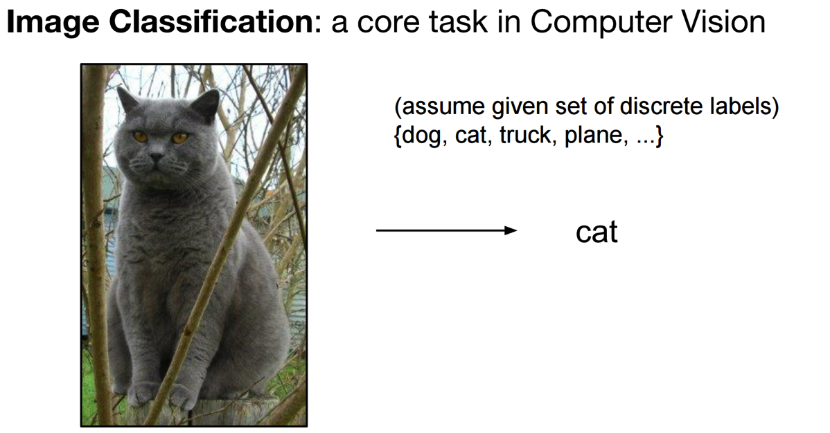
Objective:
Yes or No
A number
A sequence
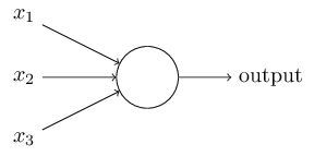
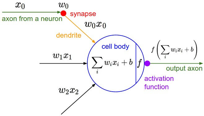
What's happend in a neural?(一个神经元的本事)
Objective:
"score"
"your performance"
"one judge"
What's happend in a neural?(一个神经元的本事)
"a bunch guys' show"
Objective:
"scores"
"one judge"
What's happend in a neural?(一个神经元的本事)
ReLU
Objective:
"a bunch guys' show"
"one judge"
"scores"
Generalize to one layer of neural(层状的神经元)
Objective:
"score"
"10 judges"
"your performance"
Generalize to one layer of neural(层状的神经元)
Objective:
"10 judges"
"scores"
"a bunch guys' show"
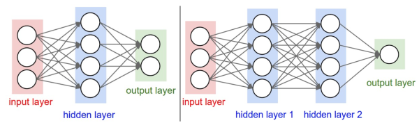
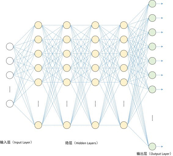
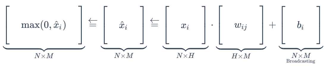
Fully-connected neural layers(全连接的神经元层)
Objective:
In each layer:
input
output
num of neurals in this layer
Draw how one sample data flows
And how the shape of data changs.
Objective:
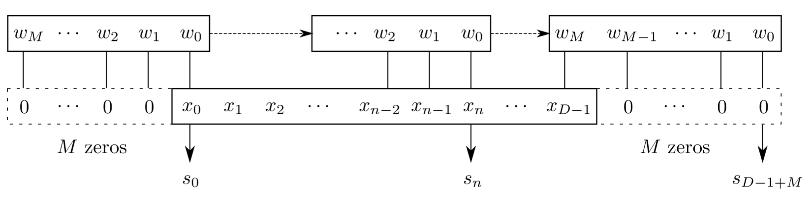
Convolution is a specialized kind of linear operation.(卷积层是全连接层的一种特例)
Objective:
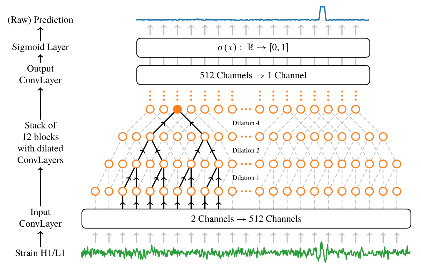
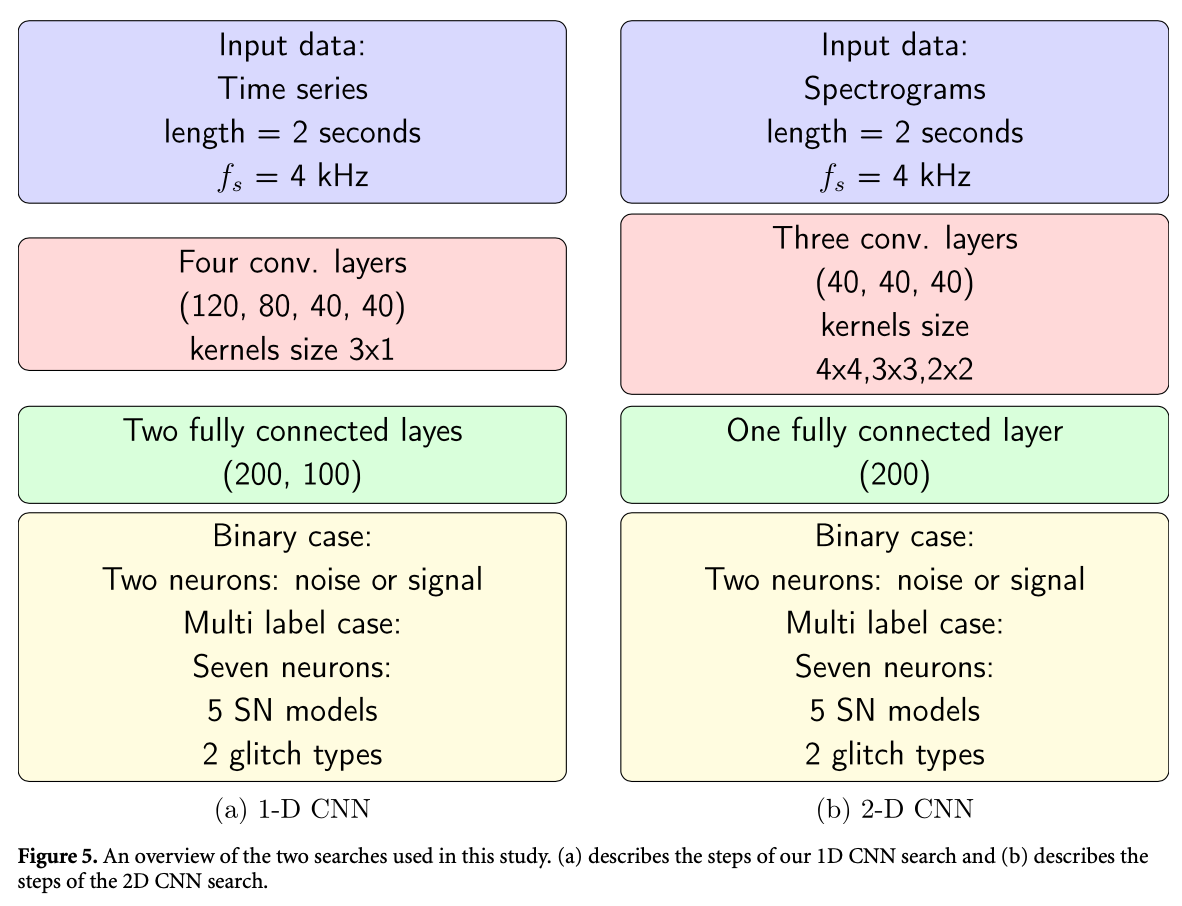
Neural networks in academic papers.(GW文献中的神经网络)
PRD. 100, 063015 (2019)
Mach. Learn.: Sci. Technol. 1 025014 (2020)
2003.09995
Expert Systems With Applications 151 (2020) 113378
"All of the current GW ML parameter estimation studies are still at the proof-of-principle stage" [2005.03745]
Real-time regression
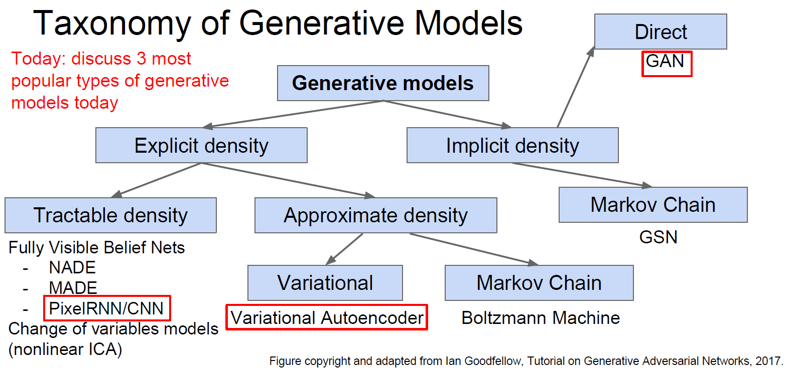
Explicit posteriors density
Suppose we have a posterior distribution \(p_{true}(x|y)\). (\(y\) is the GW data, \(x\) is the corresponding parameters)
fixed; costly sampling required
fixed; costly sampling required
Bayes' theorem
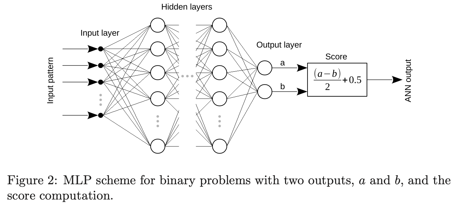
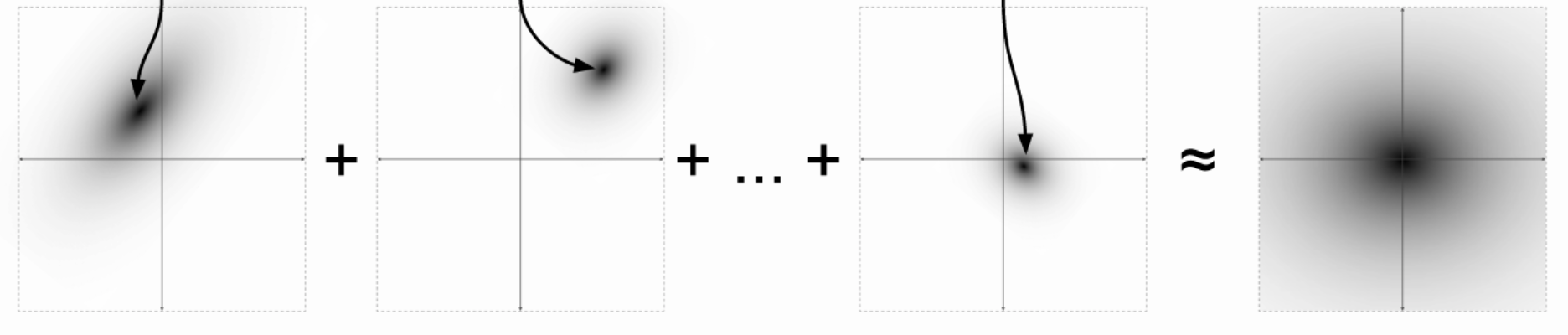
Chua et al. [PRL, 2020, 124, 041102] assume a multivariate normal distribution with weights:
NN
Suppose we have a posterior distribution \(p_{true}(x|y)\). (\(y\) is the GW data, \(x\) is the corresponding parameters)
fixed; costly sampling required
Bayes' theorem
Chua et al. [PRL, 2020, 124, 041102] assume a multivariate normal distribution with weights:
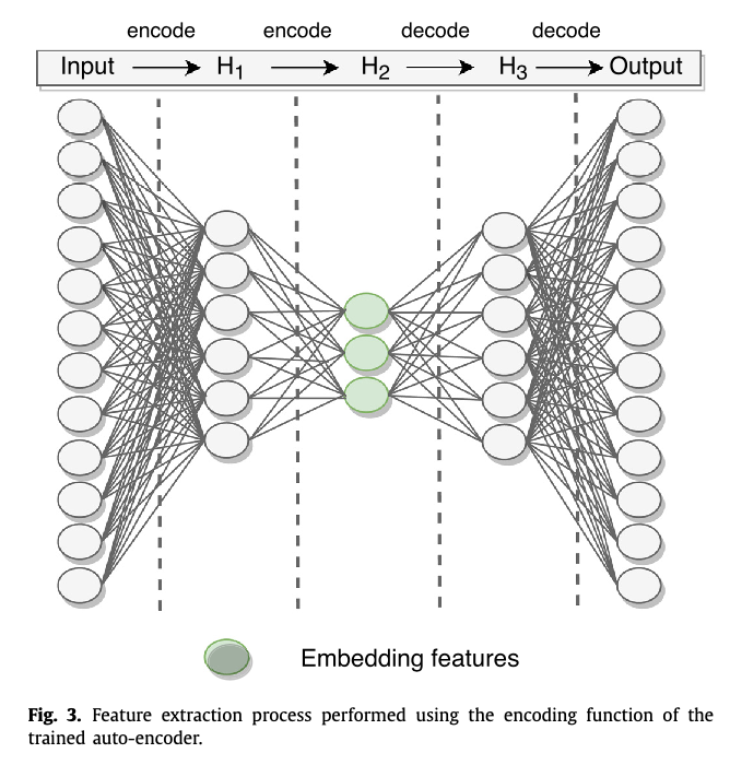
Gabbard et al. [1909.06296] (CVAE)
NN
NN
NN
NN
Suppose we have a posterior distribution \(p_{true}(x|y)\). (\(y\) is the GW data, \(x\) is the corresponding parameters)
fixed; costly sampling required
Bayes' theorem
Chua et al. [PRL, 2020, 124, 041102] assume a multivariate normal distribution with weights:
NN
Gabbard et al. [1909.06296] (CVAE)
NN
NN
NN
Green et al. [2002.07656] (MAF, CVAE+)
Suppose we have a posterior distribution \(p_{true}(x|y)\). (\(y\) is the GW data, \(x\) is the corresponding parameters)
CVAE (Train)
\(Y\) (·, 256)
\(X\) (·, 5)
KL
E2
E1
\(X'\) (·, 5)
D
(2, 8)
FYI: if dims of latent space is 2, i.e.
sample \(z\) from \(\mathcal{N}\left(\vec{\mu}, \boldsymbol{\Sigma}^{2}\right)\)
\(Y\) (·, 256)
(1, 8)
Training set: \(N=10^6\)
batchsize = 512
(·, 8)
\([(\mu_{m_1}, \sigma_{m_1}), ...]\)
\(X_1\)
\(X_2\)
\(X_n\)
latent space
strain
params
CVAE: conditional variational autoencoder
\(Y\) (·, 256)
\(X\) (·, 5)
KL
E2
E1
\(X'\) (·, 5)
D
(2, 8)
FYI: if dims of latent space is 2, i.e.
sample \(z\) from \(\mathcal{N}\left(\vec{\mu}, \boldsymbol{\Sigma}^{2}\right)\)
\(Y\) (·, 256)
(1, 8)
Training set: \(N=10^6\)
batchsize = 512
(·, 8)
\([(\mu_{m_1}, \sigma_{m_1}), ...]\)
\(X_1\)
\(X_2\)
\(X_n\)
latent space
strain
params
P
P
Q
CVAE (Train)
Objective: maximise \(L_{ELBO}\) (与数据点 X 相关联的变分下界)
ELBO: Evidence Lower Bound
CVAE: conditional variational autoencoder
FYI: if dims of latent space is 2, i.e.
\(X_1\)
\(X_2\)
\(X_n\)
latent space
CVAE (Test)
\(Y\) (·, 256)
E1
\(X'\) (·, 5)
D
sample \(z\) from \(\mathcal{N}\left(\vec{\mu}, \boldsymbol{\Sigma}^{2}\right)\)
\(Y\) (·, 256)
(1, 8)
Training set: \(N=10^6\)
batchsize = 512
(·, 8)
\([(\mu_{m_1}, \sigma_{m_1}), ...]\)
strain
P
(2, 8)
P
Objective: maximise \(L_{ELBO}\) (与数据点 X 相关联的变分下界)
ELBO: Evidence Lower Bound
CVAE: conditional variational autoencoder
\(Y\) (·, 256)
\(X\) (·, 5)
KL
E2
E1
\(X'\) (·, 5)
D
(2, 8)
sample \(z\) from \(\mathcal{N}\left(\vec{\mu}, \boldsymbol{\Sigma}^{2}\right)\)
\(Y\) (·, 256)
(1, 8)
Training set: \(N=10^6\)
batchsize = 512
(·, 8)
\([(\mu_{m_1}, \sigma_{m_1}), ...]\)
strain
params
Objective: maximise \(L_{ELBO}\) (与数据点 X 相关联的变分下界)
P
P
Q
CVAE
Drawbacks:
Mystery:
The final slice. 💪
ELBO: Evidence Lower Bound
CVAE: conditional variational autoencoder
By He Wang
Abstract: Firstly, I will talk about some basic concepts of deep neural networks and I hope it would help clear up misunderstandings and rumors related to understand how a neural network works, etc. Then, based on these concepts, I will try to briefly review the current GW ML parameter estimation studies (1903.01998, 1909.06296, PRL(2020) 124 041102, 2002.07656, 2008.03312; selected), especially how they try to built up a neural network to estimate the posterior distribution. The relative drawbacks and mysteries of their works are also mentioned.


