


He Wang PRO
Knowledge increases by sharing but not by saving.
He Wang (王赫)
Institute of Theoretical Physics, CAS
Beijing Normal University
on behalf of the KAGRA collaboration
7th KAGRA International Workshop , 15:45-16:05 Asia/Taipei on December 19\(^\text{th}\), 2020
Based on DOI: 10.1103/physrevd.101.104003
hewang@mail.bnu.edu.cn / hewang@itp.ac.cn
Collaborators:
Zhoujian Cao (BNU)
Shichao Wu (BNU)
Xiaolin Liu (BNU)
Jian-Yang Zhu (BNU)
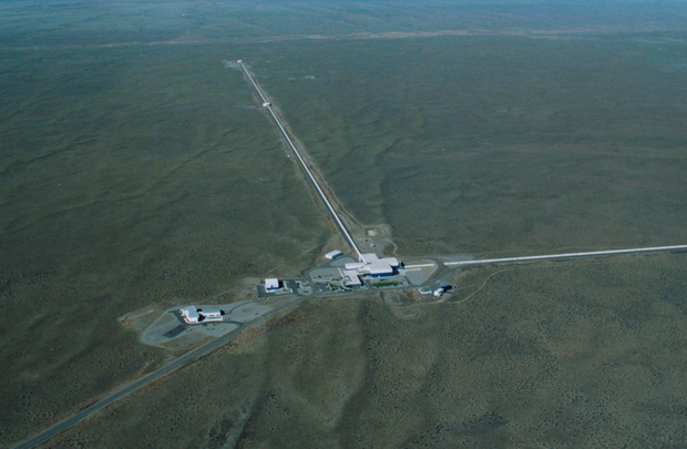
LIGO Hanford (H1)
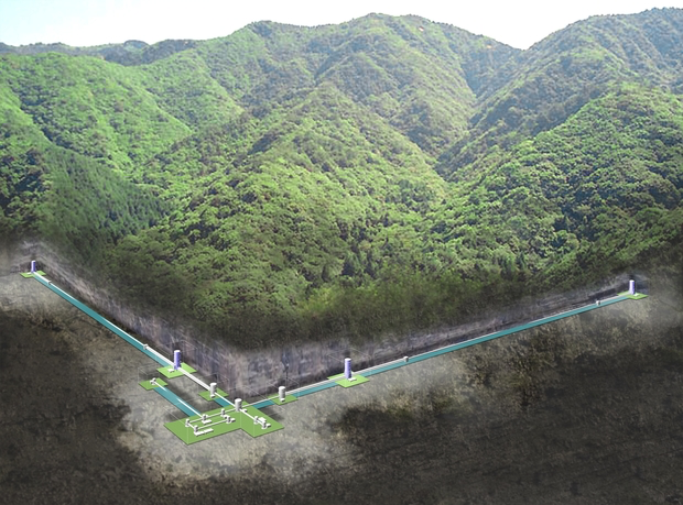
KAGRA
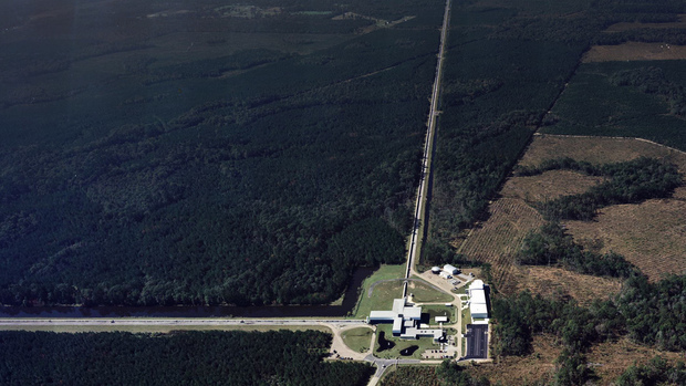
LIGO Livingston (L1)
Noise power spectral density (one-sided)
where
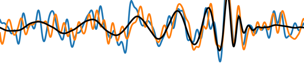
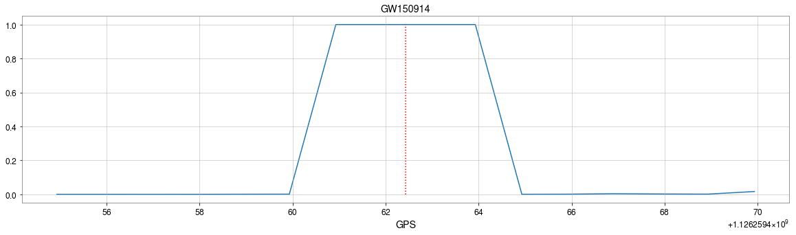
The template that best matches GW150914 event
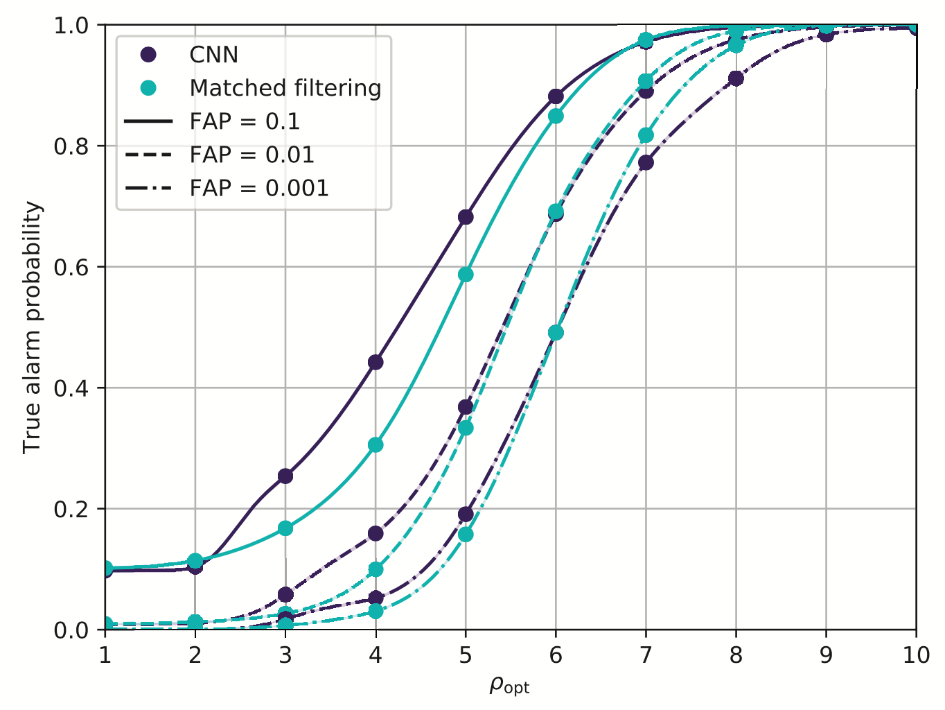
Proof-of-principle studies
Production search studies
Milestones
More related works, see Survey4GWML (https://iphysresearch.github.io/Survey4GWML/)
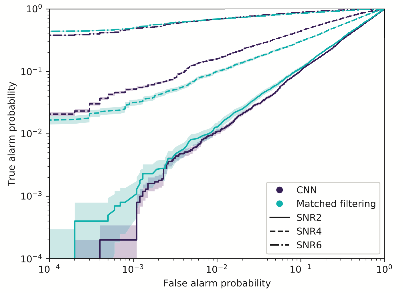
Resilience to real non-Gaussian noise (Robustness)
Acceleration of existing pipelines (Speed, <0.1ms)
Stimulated background noises
Classification
Feature extraction
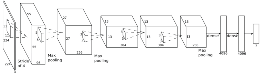
Convolutional Neural Network (ConvNet or CNN)
A specific design of the architecture is needed.
A specific design of the architecture is needed.
Classification
Feature extraction
Convolutional Neural Network (ConvNet or CNN)
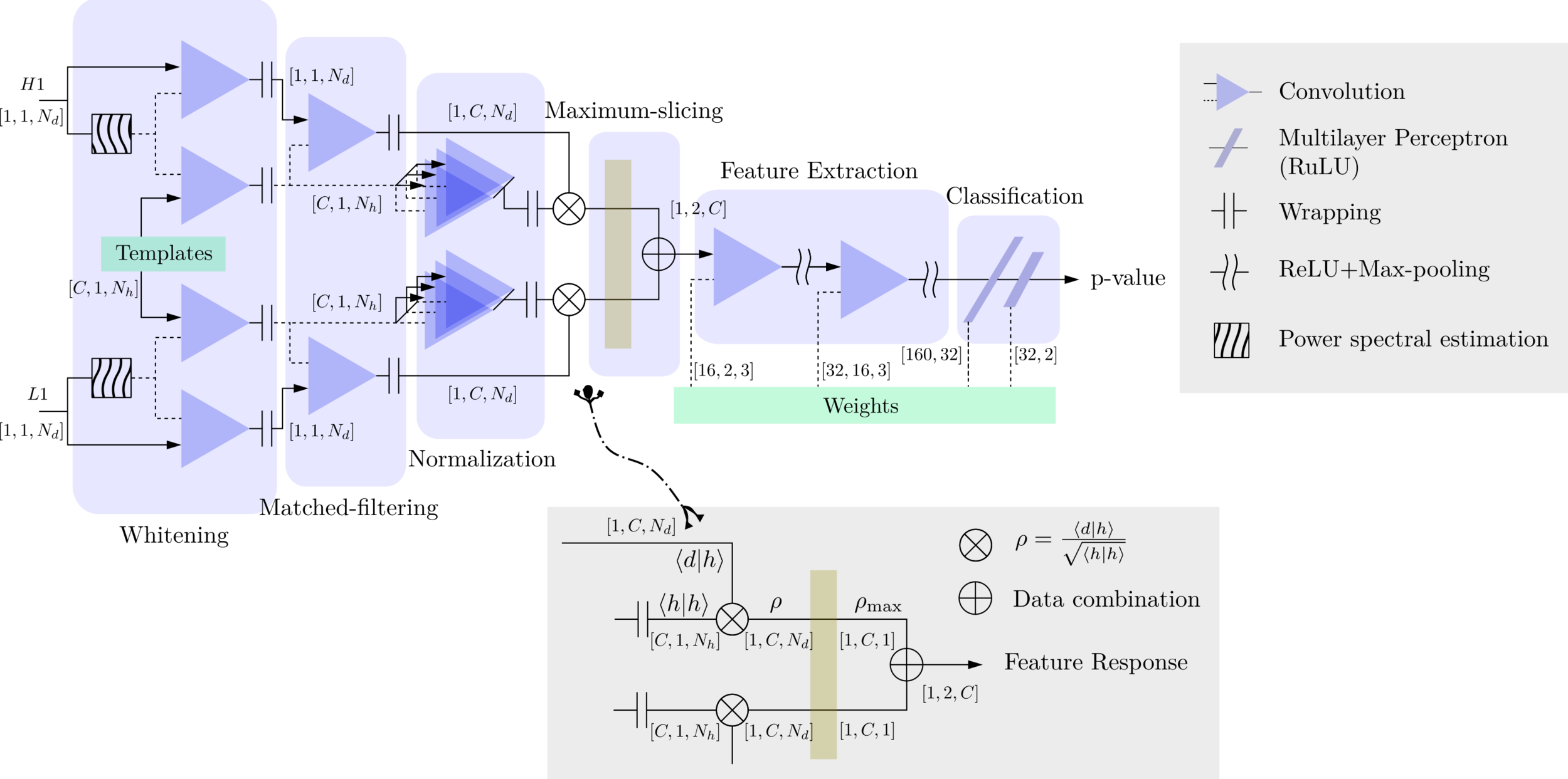
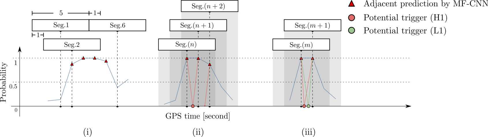
MFCNN
MFCNN
MFCNN
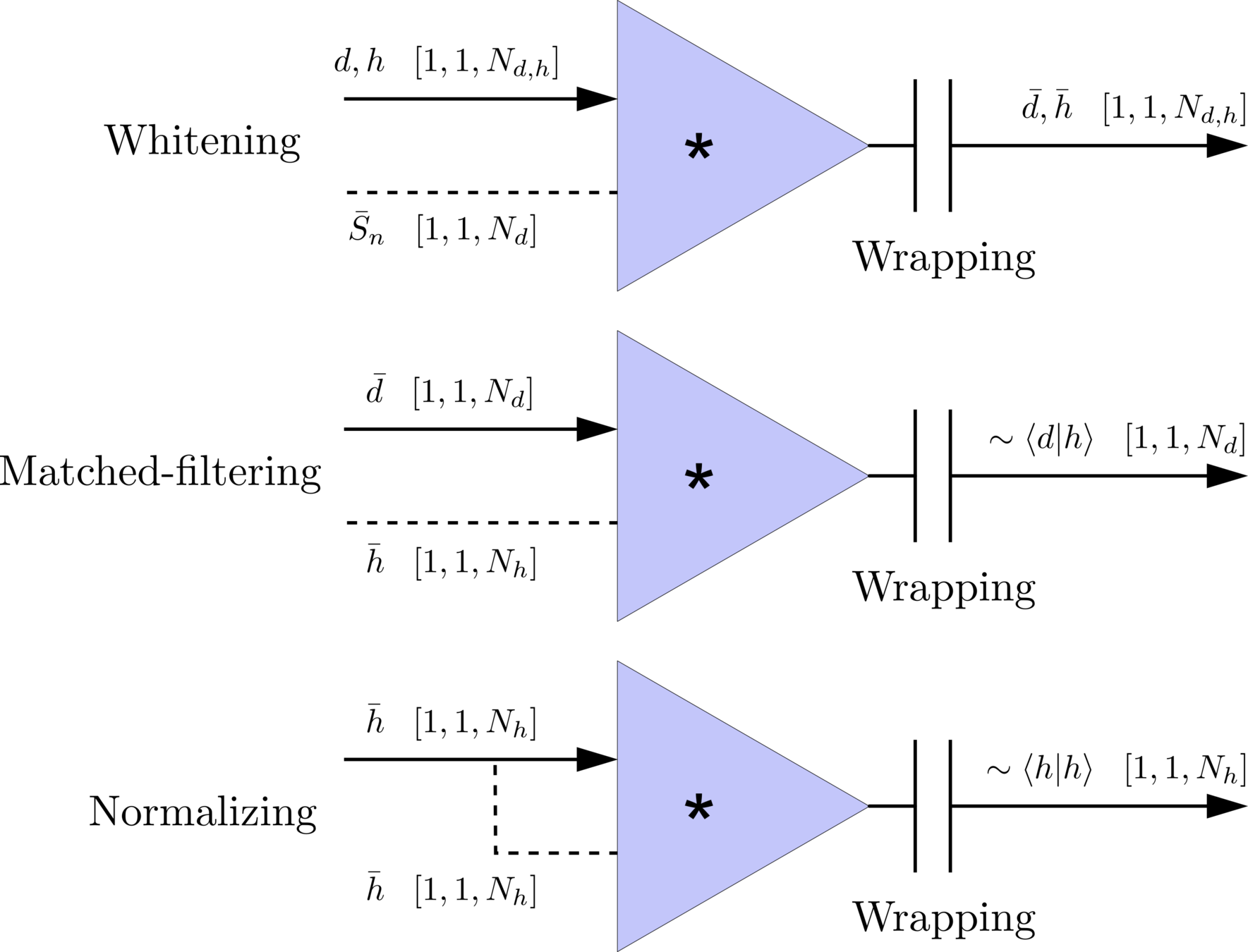
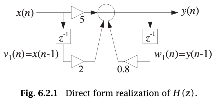
Matched-filtering (cross-correlation with the templates) can be regarded as a convolutional layer with a set of predefined kernels.
>> Is it matched-filtering ?
>> Wait, It can be matched-filtering!
Classification
Feature extraction
Convolutional Neural Network (ConvNet or CNN)
Frequency domain
\(S_n(|f|)\) is the one-sided average PSD of \(d(t)\)
(whitening)
where
Time domain
Frequency domain
(normalizing)
(matched-filtering)
\(S_n(|f|)\) is the one-sided average PSD of \(d(t)\)
(whitening)
where
Time domain
Frequency domain
(normalizing)
(matched-filtering)
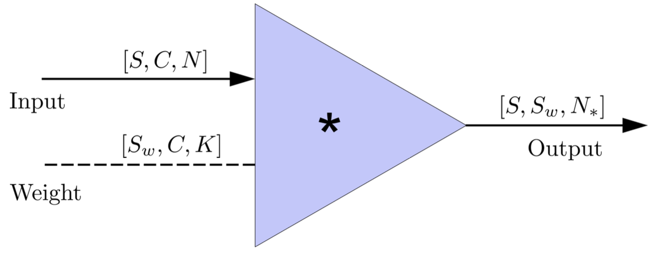
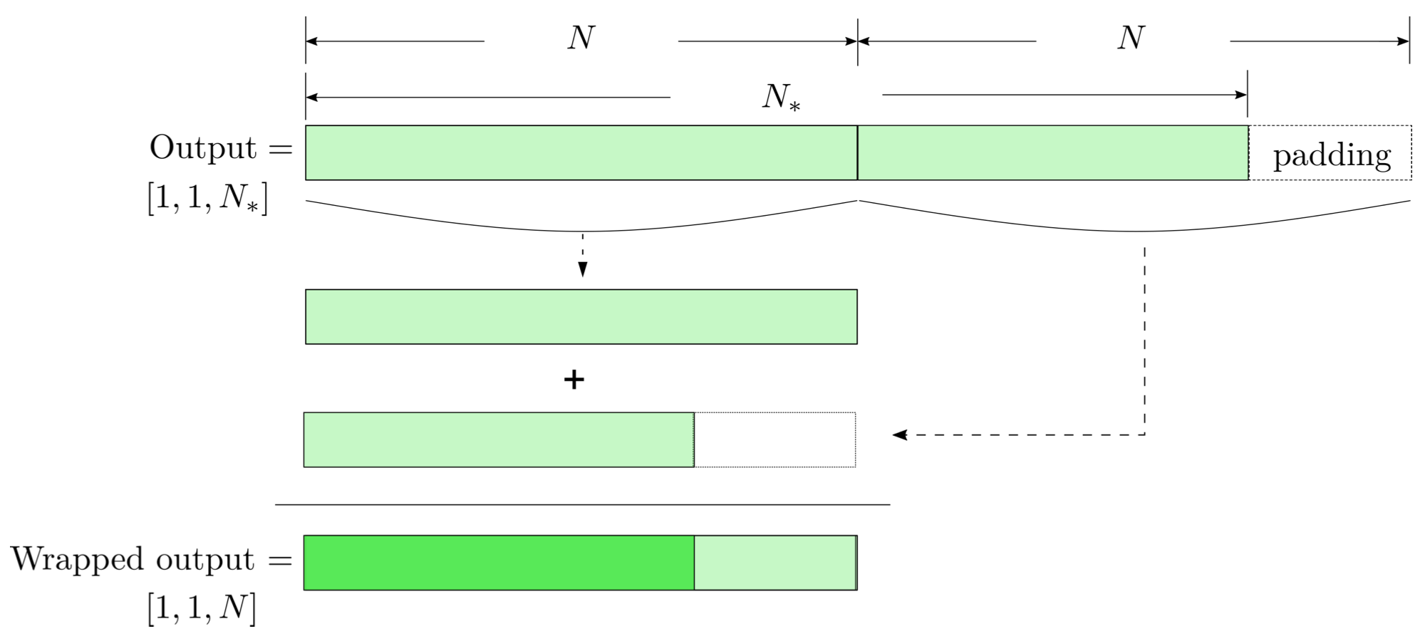
FYI: \(N_\ast = \lfloor(N-K+2P)/S\rfloor+1\)
(A schematic illustration for a unit of convolution layer)
Deep Learning Framework
\(S_n(|f|)\) is the one-sided average PSD of \(d(t)\)
(whitening)
where
Time domain
Frequency domain
(normalizing)
(matched-filtering)
Deep Learning Framework
modulo-N circular convolution
Input
Output
Input
Output
Input
Output
import mxnet as mx
from mxnet import nd, gluon
from loguru import logger

def MFCNN(fs, T, C, ctx, template_block, margin, learning_rate=0.003):
    logger.success('Loading MFCNN network!')
    net = gluon.nn.Sequential()
    with net.name_scope():
        net.add(MatchedFilteringLayer(mod=fs*T, fs=fs,
                                      template_H1=template_block[:,:1],
                                      template_L1=template_block[:,-1:]))
        net.add(CutHybridLayer(margin = margin))
        net.add(Conv2D(channels=16, kernel_size=(1, 3), activation='relu'))
        net.add(MaxPool2D(pool_size=(1, 4), strides=2))
        net.add(Conv2D(channels=32, kernel_size=(1, 3), activation='relu'))
        net.add(MaxPool2D(pool_size=(1, 4), strides=2))
        net.add(Flatten())
        net.add(Dense(32))
        net.add(Activation('relu'))
        net.add(Dense(2))
	# Initialize parameters of all layers
    net.initialize(mx.init.Xavier(magnitude=2.24), ctx=ctx, force_reinit=True)
    return net
The available codes: https://gist.github.com/iphysresearch/a00009c1eede565090dbd29b18ae982c
1 sec duration
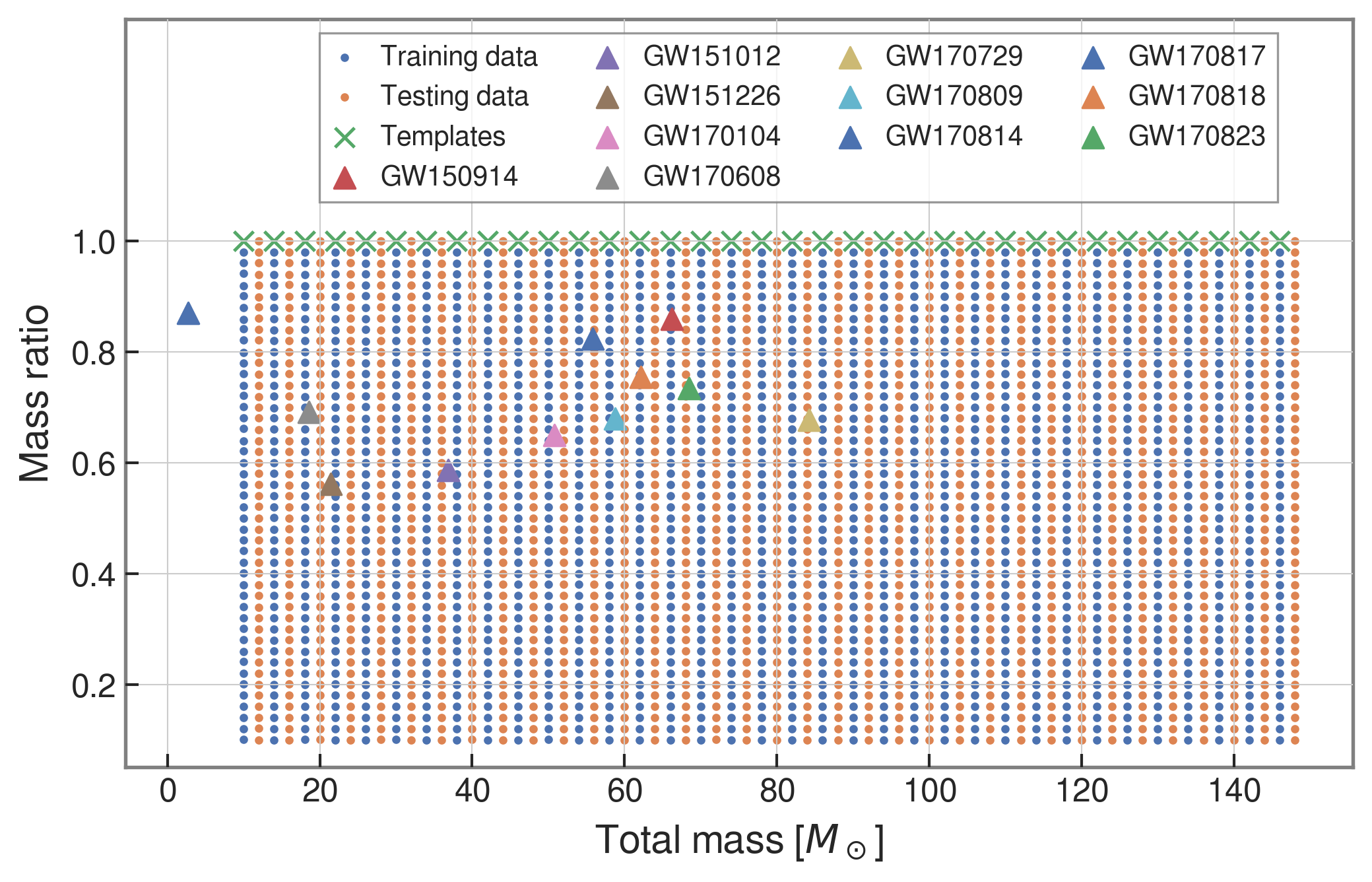
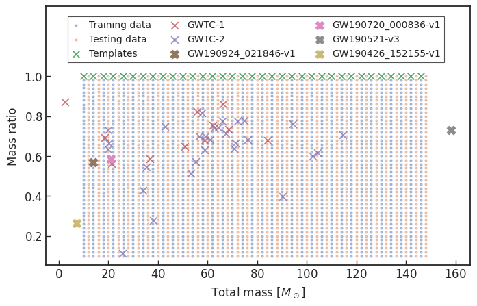
35 templates used
FYI: sampling rate = 4096Hz
| templates | waveforms (train/test) | |
|---|---|---|
| Number | 35 | 1610 |
| Length (sec) | 1 | 5 |
| equal mass |
FYI: sampling rate = 4096Hz
| templates | waveforms (train/test) | |
|---|---|---|
| Number | 35 | 1610 |
| Length (sec) | 1 | 5 |
| equal mass |
input
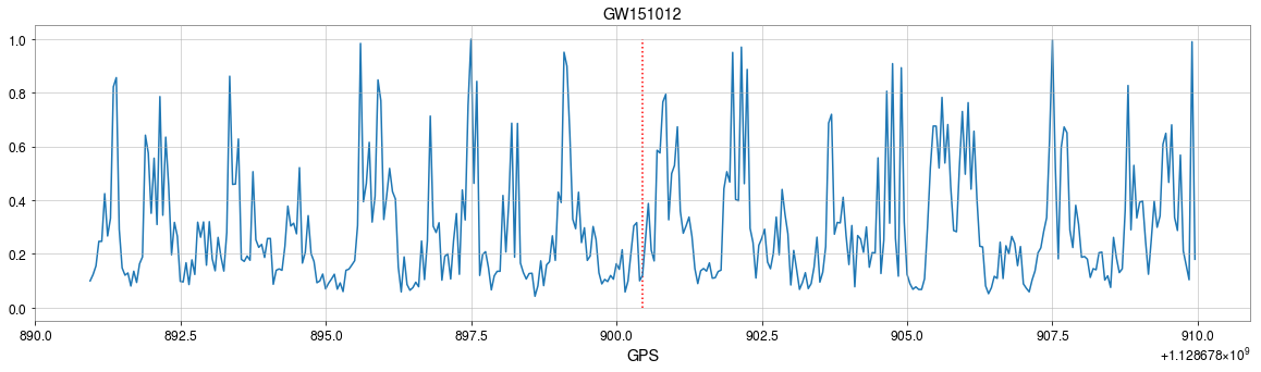
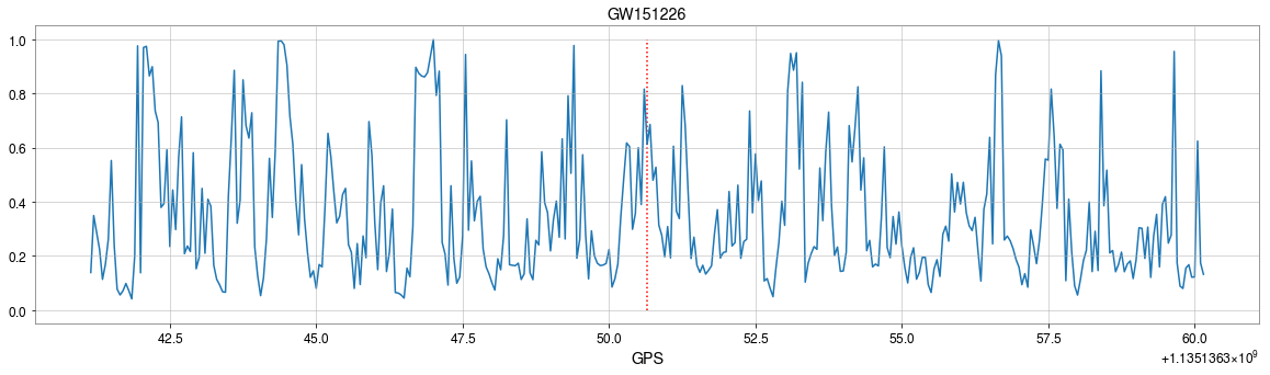
GW170817
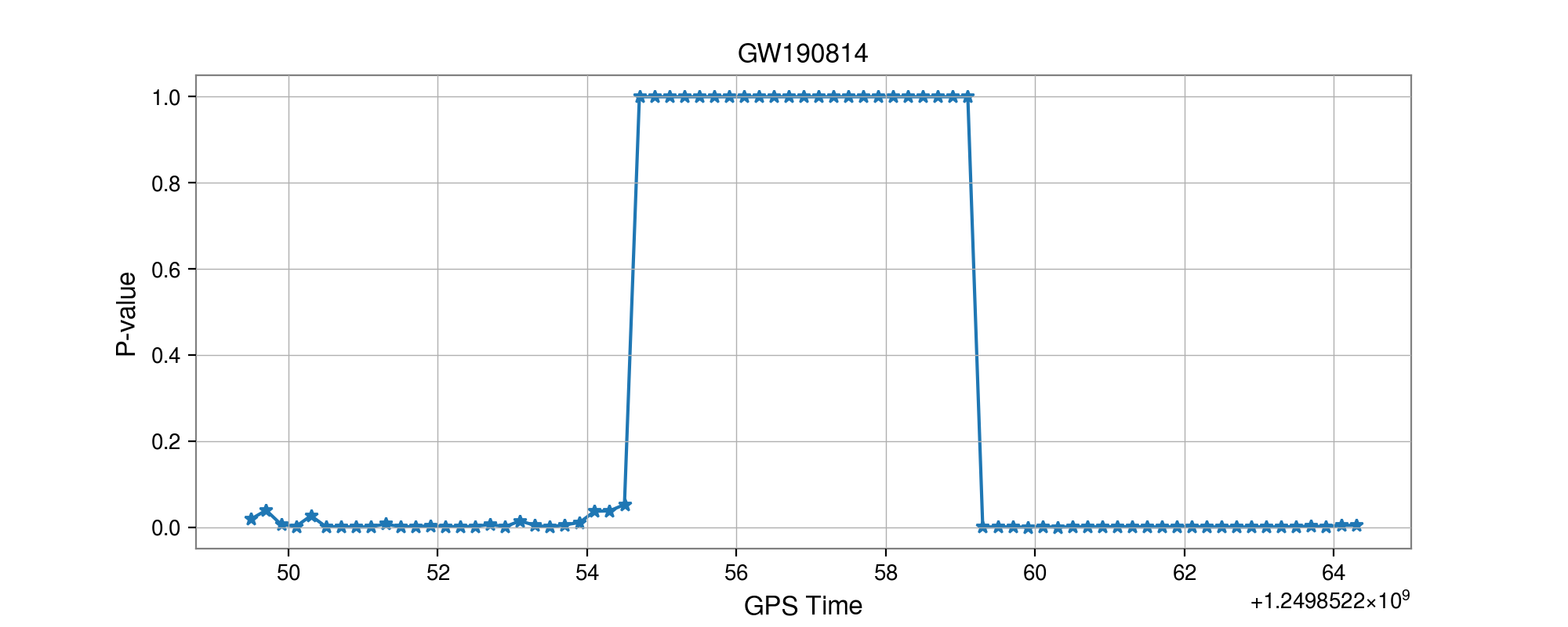
GW190814
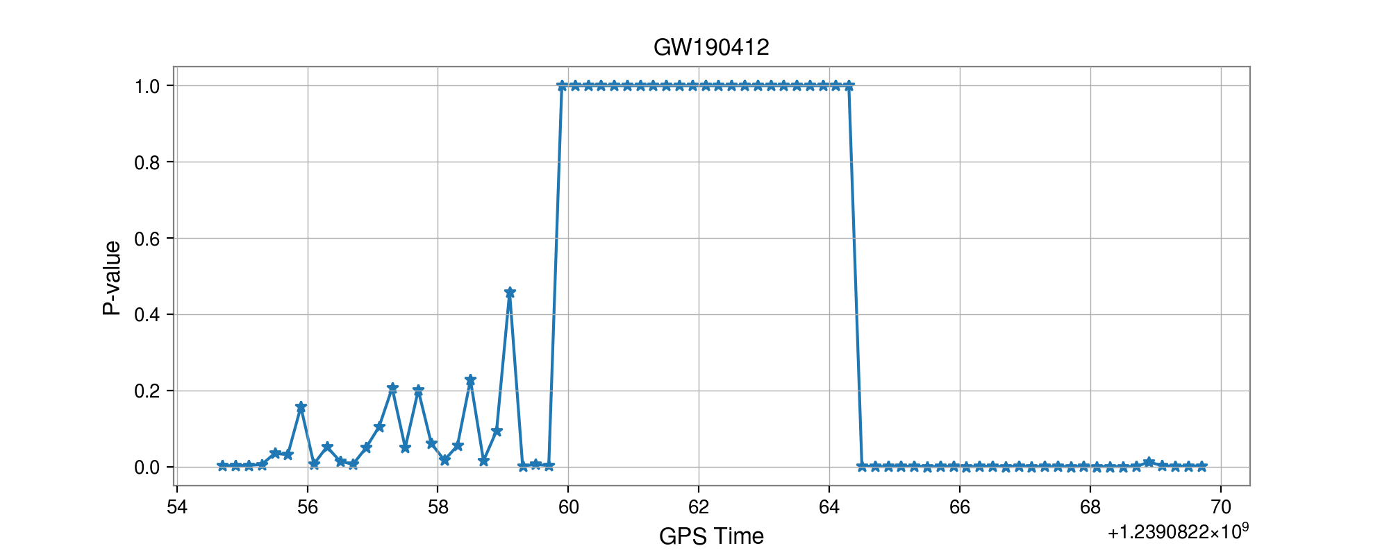
GW190412
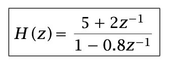
An example of transfer function:
CNN
RNN
Softmax function:
Score
Pred.
This slide: https://slides.com/iphysresearch/kiw7
for _ in range(num_of_audiences):
    print('Thank you for your attention! 🙏')
A example of Transfer function:
Softmax function:
Pred.
By He Wang
7th KAGRA International Workshop , 15:45-16:05 Asia/Taipei on December 19\(^\text{th}\), 2020


