


He Wang PRO
Knowledge increases by sharing but not by saving.
In collaboration with Prof. Dr. Zhou-Jian Cao
Webniar, July 19th, 2020
He Wang (王赫)
[hewang@mail.bnu.edu.cn]
Department of Physics, BNU
Based on: PhD thesis (HTML); 10.1103/PhysRevD.101.104003
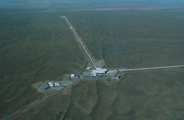
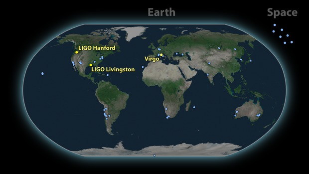
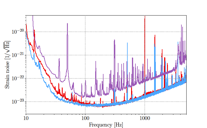
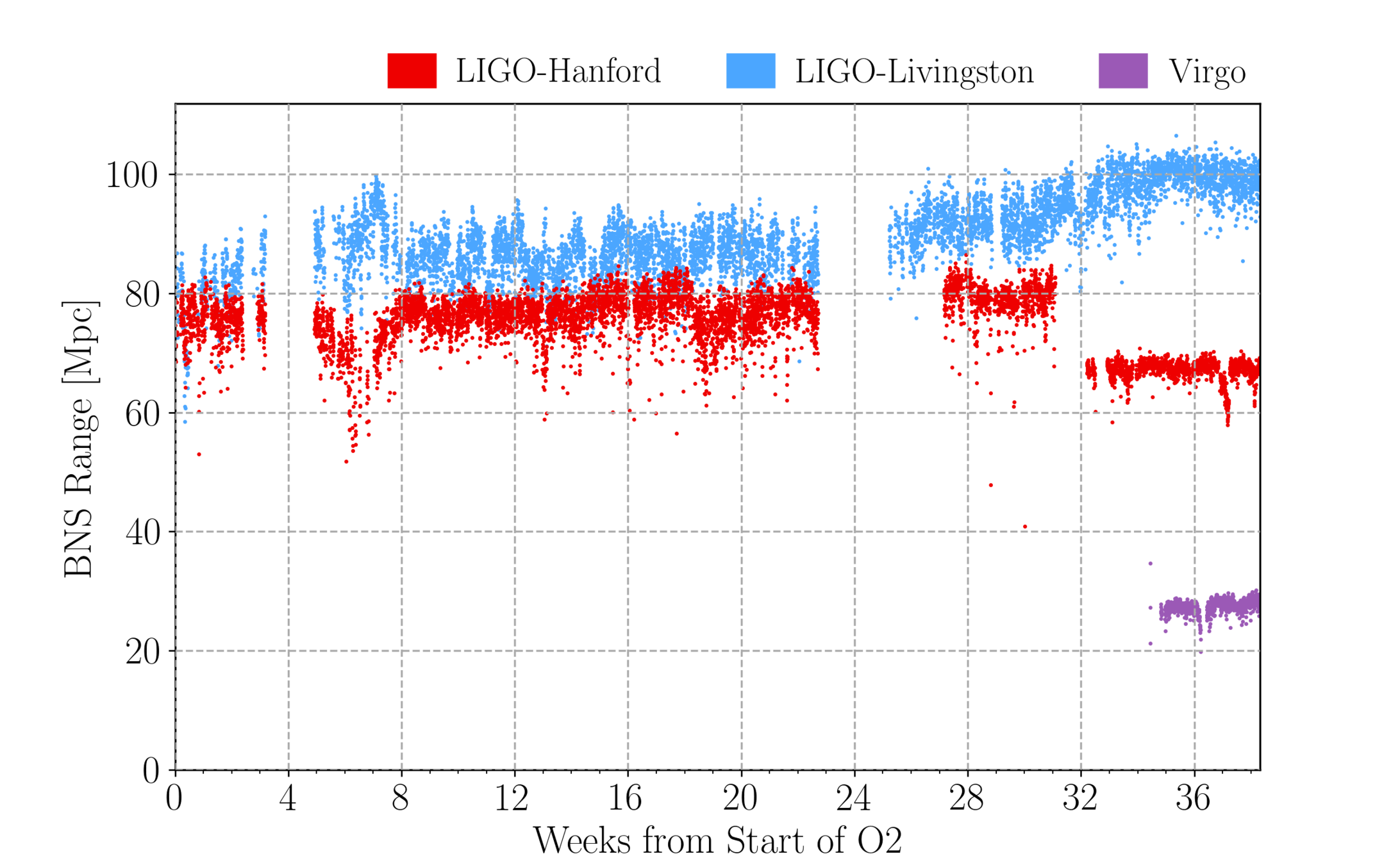
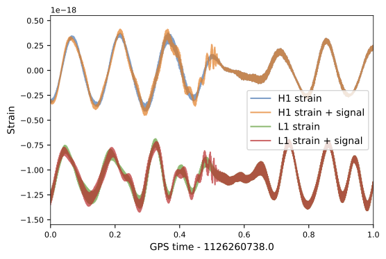
LIGO Hanford (H1)
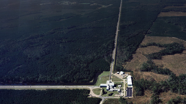
LIGO Livingston (L1)
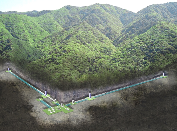
KAGRA
Observational Experiment
Theoretical Modeling
Data Analysis
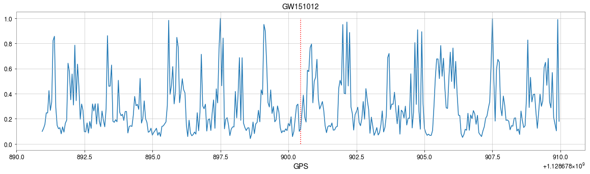
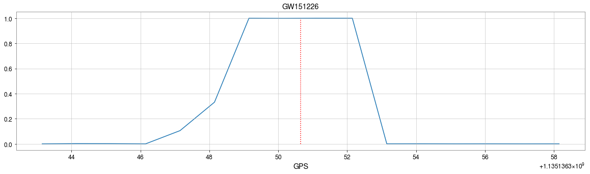
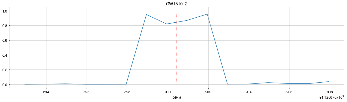
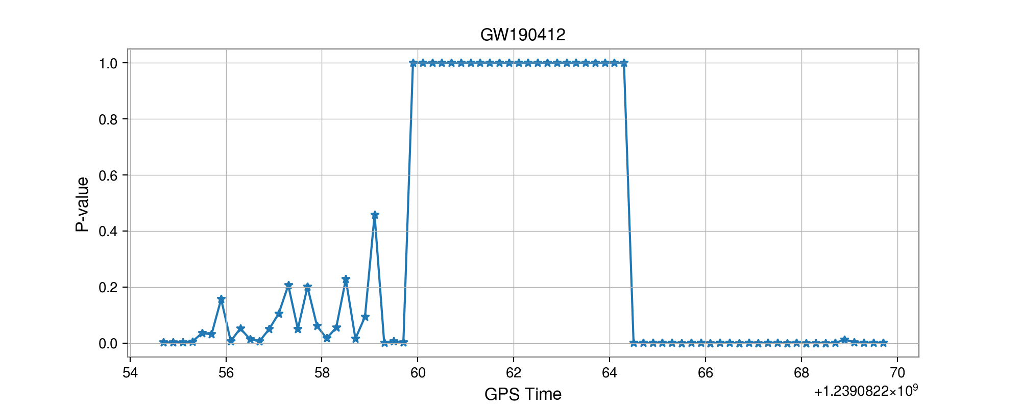
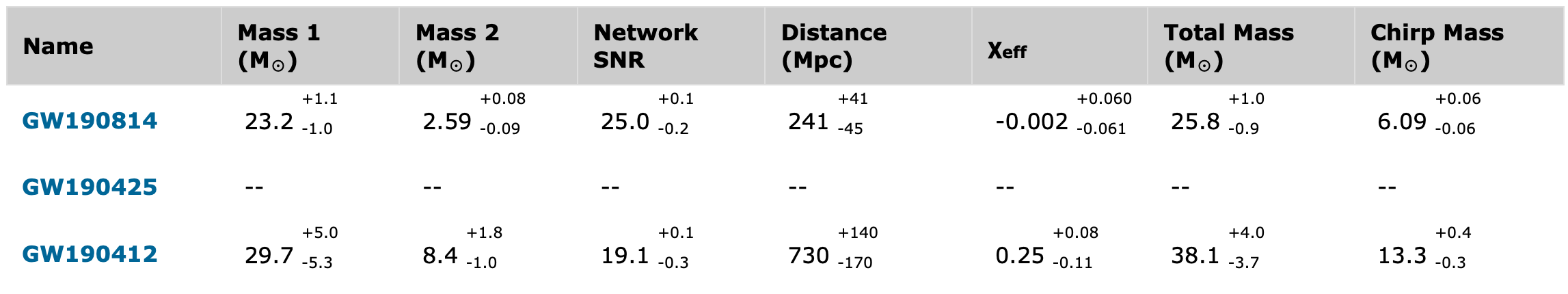
GW151012
GW170729
GW170809
GW170818
GW170823
GW170121
GW170304
GW170721
(GW151205)
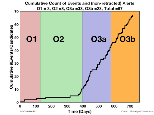
GW Event Detections
O1
O2
O3
GWTC2 (?)
2-OGC (2020)
...
Anomalous non-Gaussian transients, known as glitches
Lack of GW templates
Real-time / low-latency analysis of the raw big data
Inadequate matched-filtering method
A threshold is used on SNR value to build our templates bank with a maximum loss of 3% of its SNR.
Noise power spectral density
Matched filtering Technique:
Optimal detection technique for templates, with Gaussian and stationary detector noise.
credits G. Guidi
Anomalous non-Gaussian transients, known as glitches
Lack of GW templates
Real-time / low-latency analysis of the raw big data
Inadequate matched-filtering method
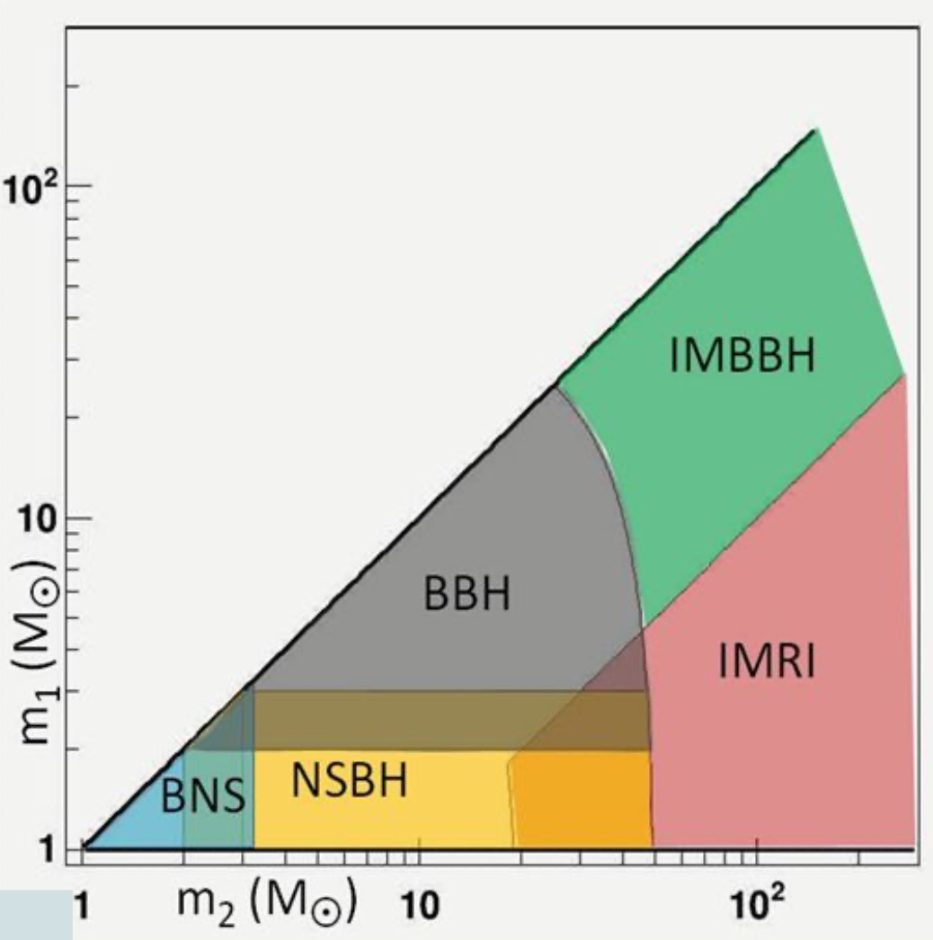
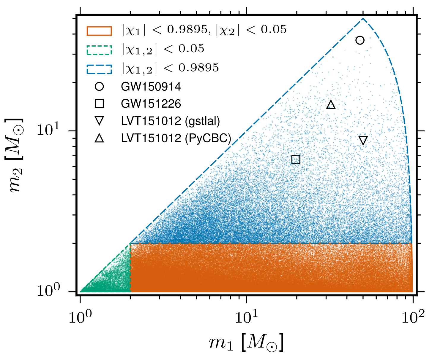
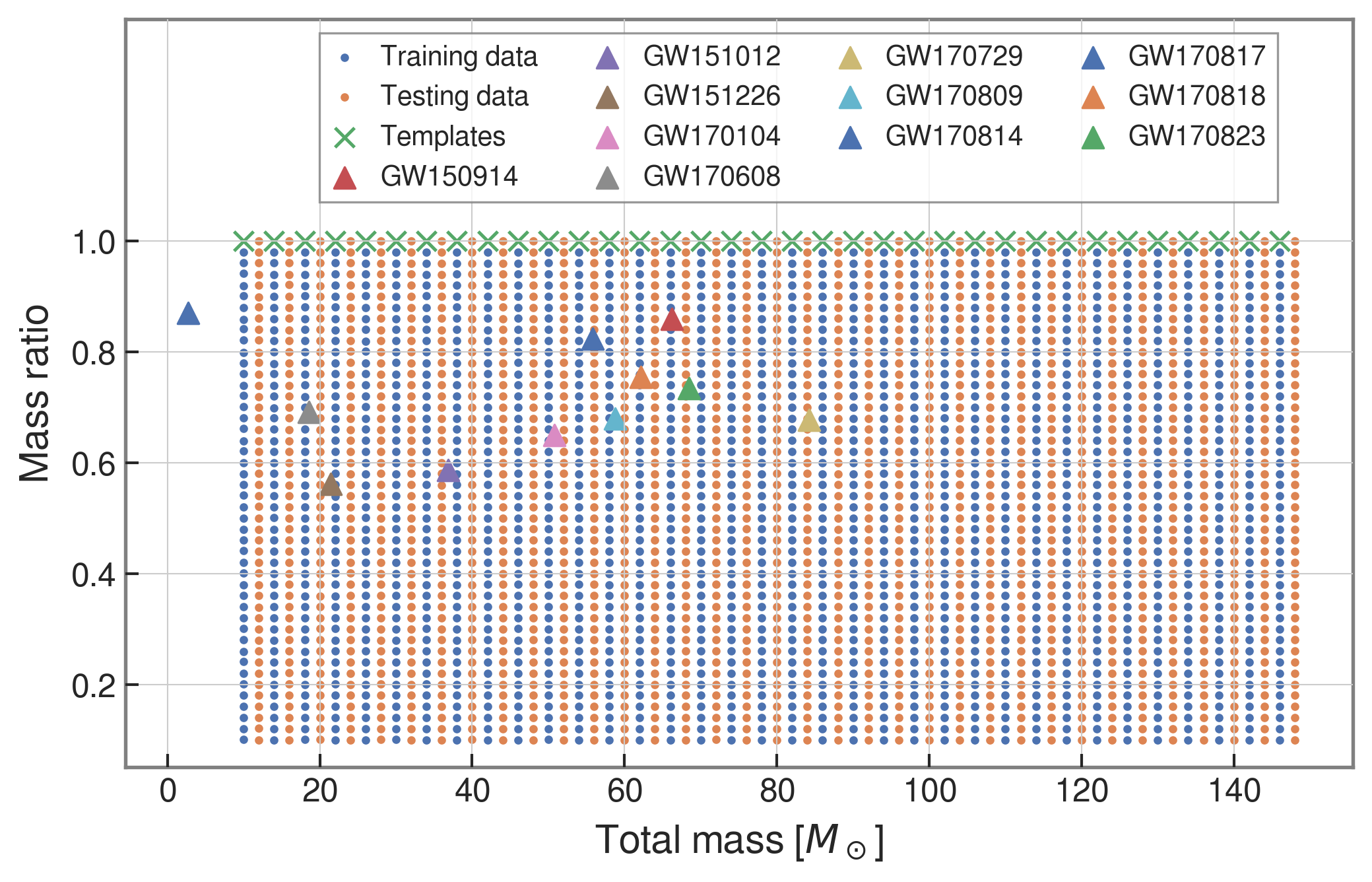
The 4-D search parameter space in O1
covered by the template bank
to circular binaries for which the spin of the systems is aligned (or antialigned) with the orbital angular momentum of the binary.
~250,000 template waveforms are used.
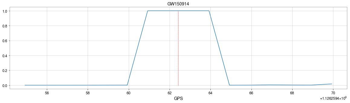
The template that best matches GW150914
Anomalous non-Gaussian transients, known as glitches
Lack of GW templates
Real-time / low-latency analysis of the raw big data
Inadequate matched-filtering method
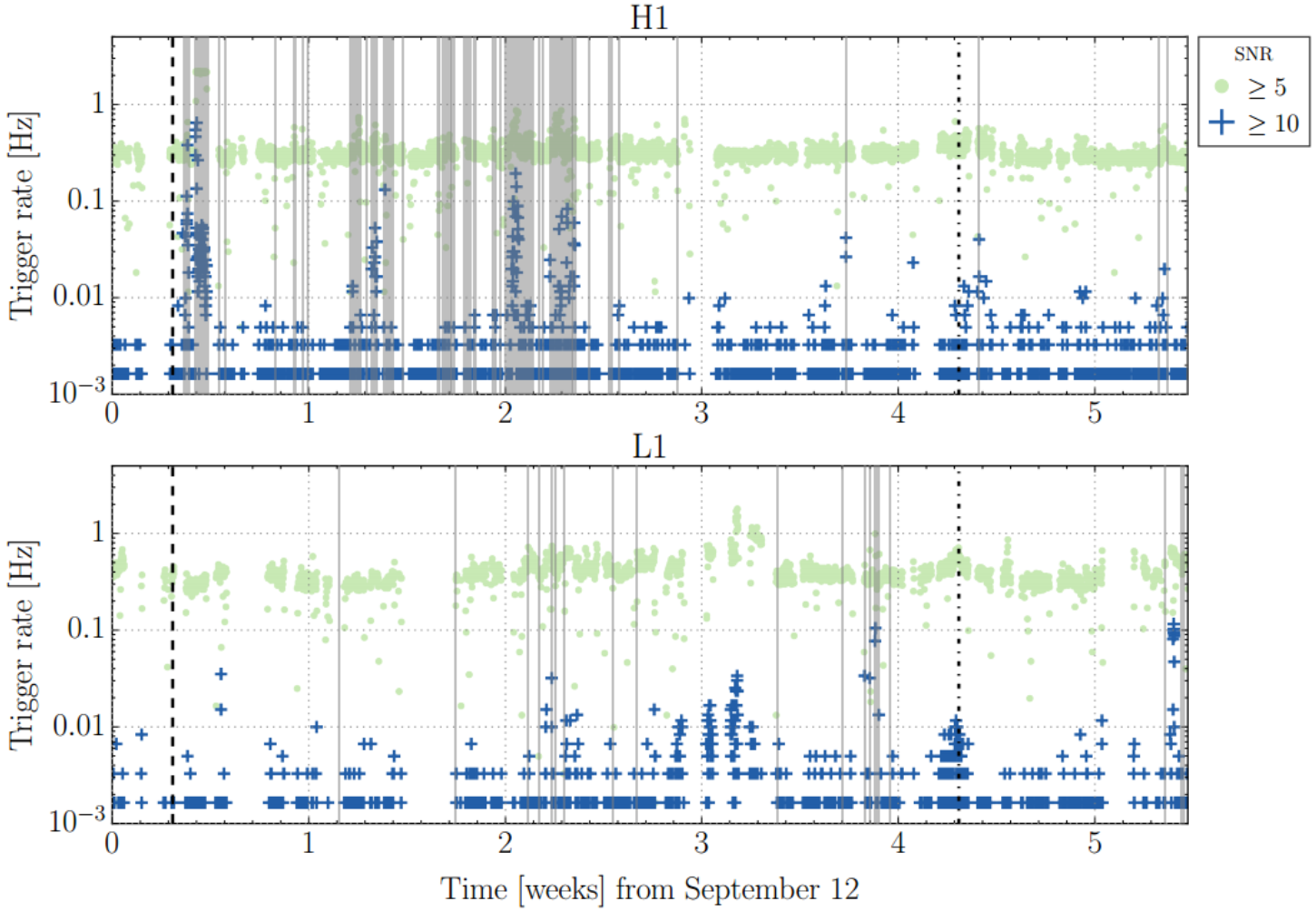
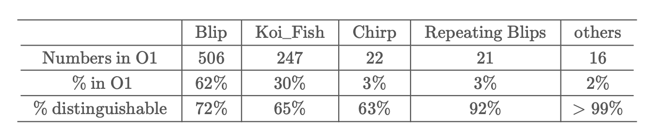
How many "trash" events?
LIGO L1 and H1 triggers rates during O1
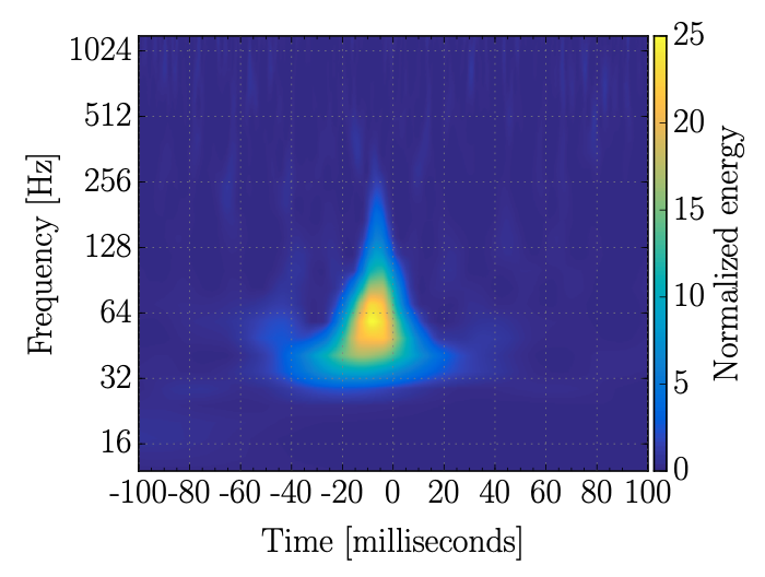
A 'blip' glitch
Anomalous non-Gaussian transients, known as glitches
Lack of GW templates
Real-time / low-latency analysis of the raw big data
Inadequate matched-filtering method
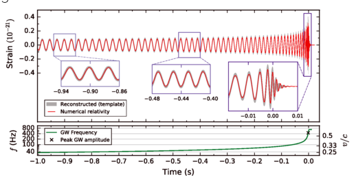
GW170817: Very long inspiral "chirp" (>100s) firmly detected by the LIGO-Virgo network,
GRB 170817A: 1.74\(\pm\)0.05s later, weak short gamma-ray burst observed by Fermi (also detected by INTEGRAL)
First LIGO-Virgo alert 27 minutes later.
Anomalous non-Gaussian transients, known as glitches
Lack of GW templates
Inadequate matched-filtering method
Covering more parameter-space (interpolation)
Automatic generalization to new sources (extrapolation)
Resilience to real non-Gaussian noise (Robustness)
Acceleration of existing pipelines
(Speed, <0.1ms)
...
Why Deep Learning ?
Proof-of-principle studies
Production search studies
Milestones
Real-time / low-latency analysis of the raw big data
More related works, see Survey4GWML (https://iphysresearch.github.io/Survey4GWML/)
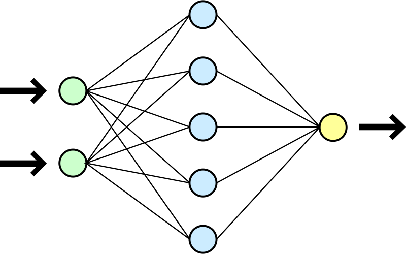
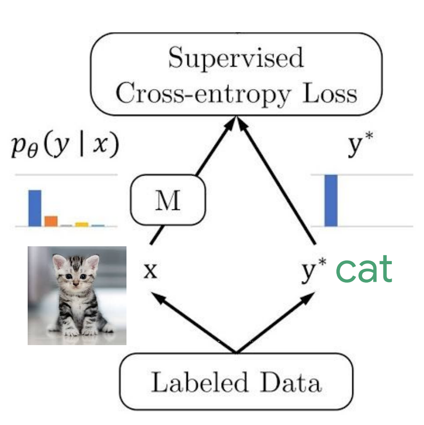
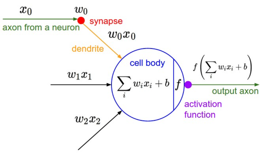
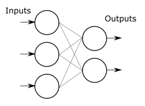
Map / Algorithm
Input
Output
A number
A sequence
Yes or No
Our model / network
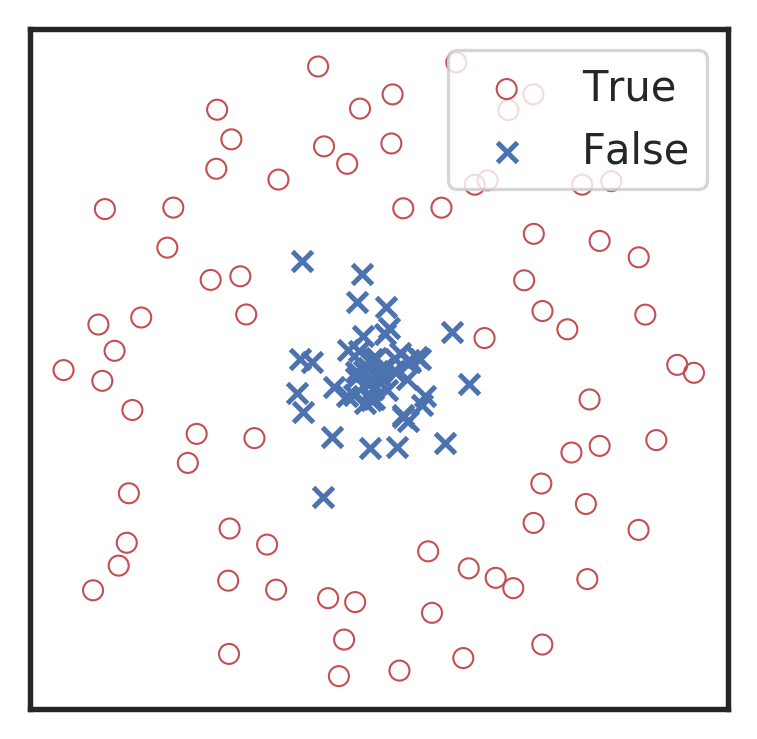
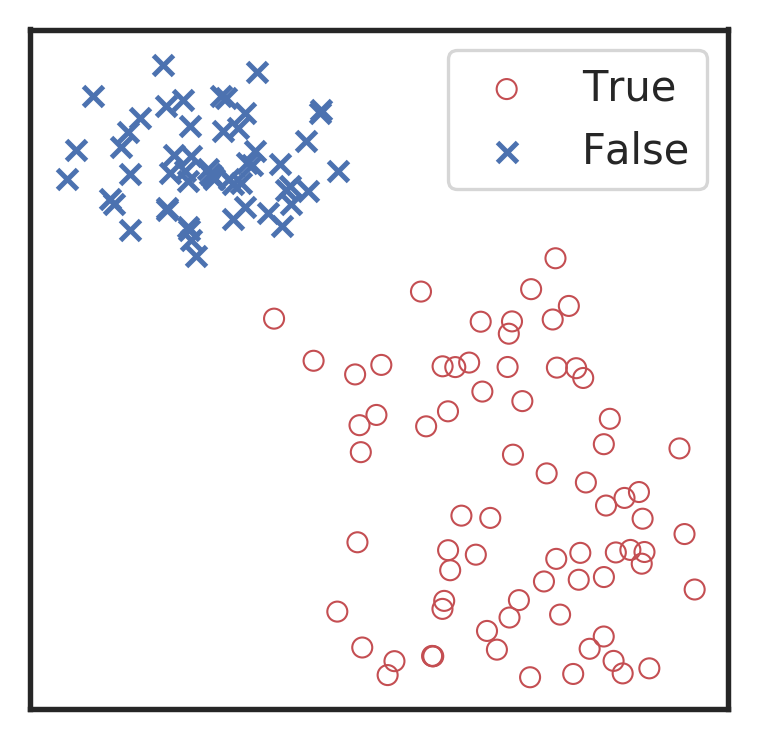
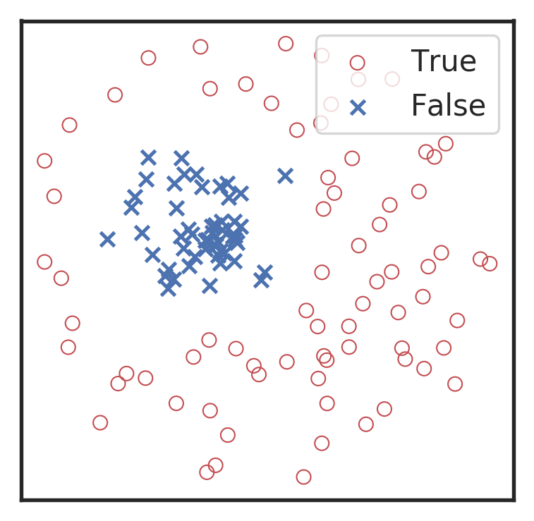
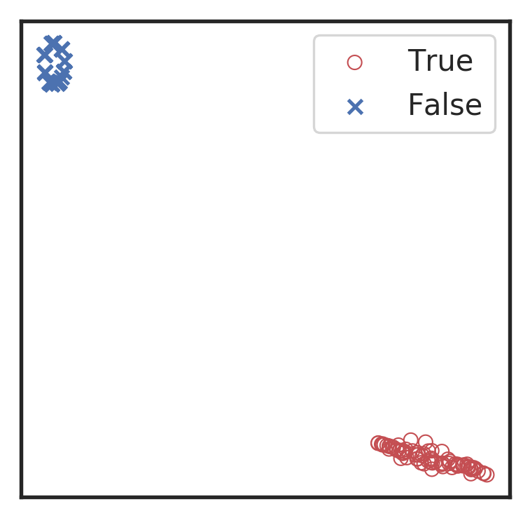
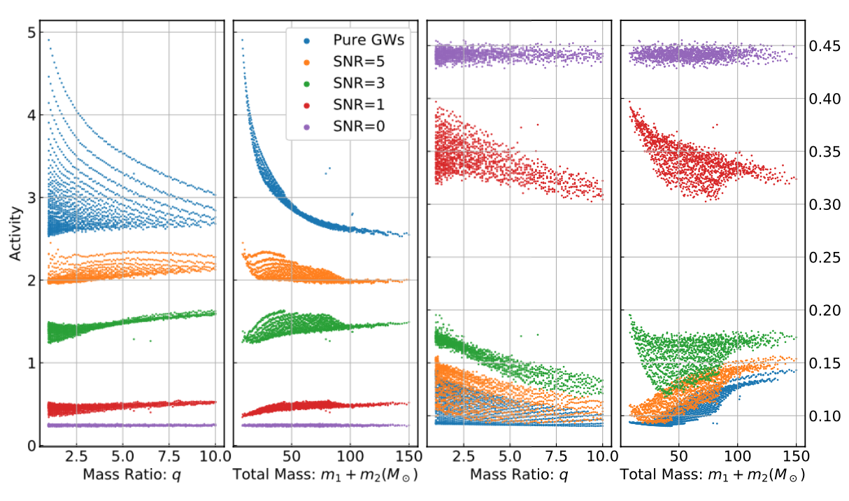
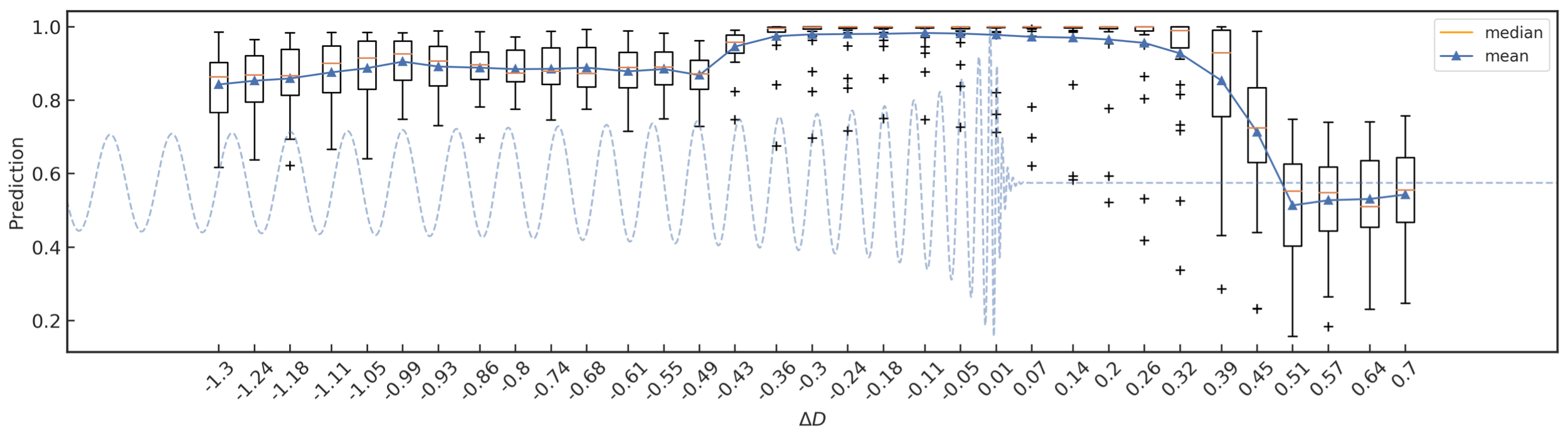
Visualization for the high-dimensional feature maps of learned network in layers for bi-class using t-SNE.
Classification
Feature extraction
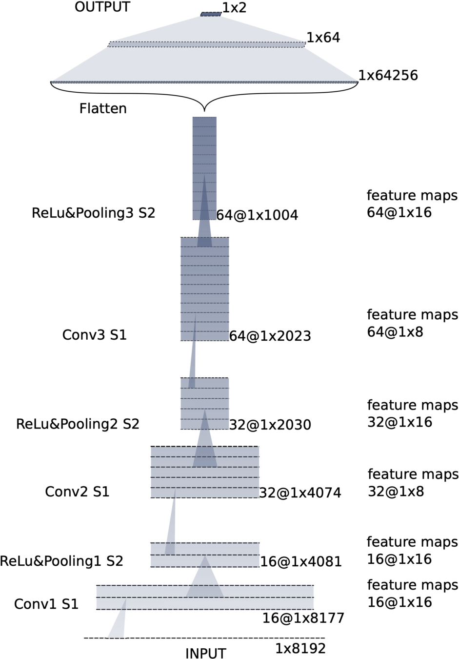
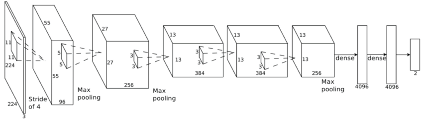
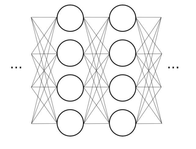
Convolutional neural network (ConvNet or CNN)
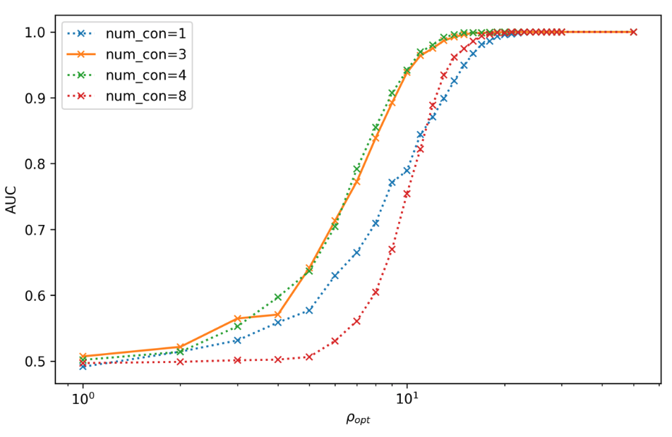
Effect of the number of the convolutional layers on signal recognizing accuracy.
Fine-tune Convolutional Neural Network
Fine-tune Convolutional Neural Network
Classification
Feature extraction
Convolutional neural network (ConvNet or CNN)
Visualization of the top activation on average at the \(3\)rd layer projected back to time domain using the deconvolutional network approach
The top activated
The top activated
Classification
Feature extraction
Convolutional neural network (ConvNet or CNN)
Marginal!
Extracted features play a decisive role.
Visualization of the top activation on average at the \(3\)rd layer projected back to time domain using the deconvolutional network approach
Classification
Feature extraction
Convolutional neural network (ConvNet or CNN)
Marginal!
Marginal!
Extracted features play a decisive role.
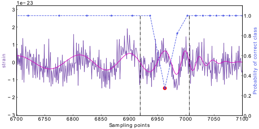
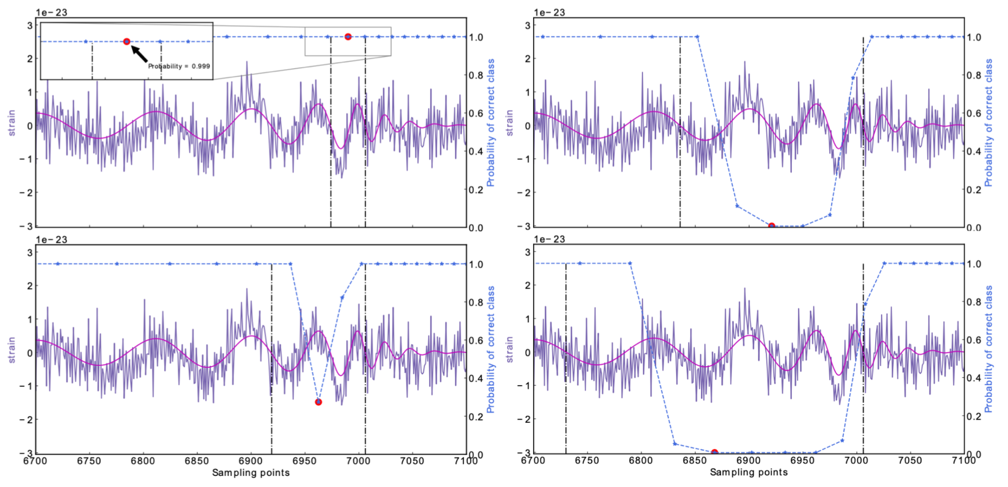
Occlusion Sensitivity
High sensitivity to the peak features of GW.
Classification
Feature extraction
Convolutional neural network (ConvNet or CNN)
Extracted features play a decisive role.
Occlusion Sensitivity
High sensitivity to the peak features of GW.
Classification
Feature extraction
Convolutional neural network (ConvNet or CNN)
Marginal!
(too sensitive against the background + hard to find the events)
A specific design of the architecture is needed.
[as Timothy D. Gebhard et al. (2019)]
Classification
Feature extraction
Convolutional neural network (ConvNet or CNN)
A specific design of the architecture is needed.
(too sensitive against the background + hard to find the events)
[as Timothy D. Gebhard et al. (2019)]
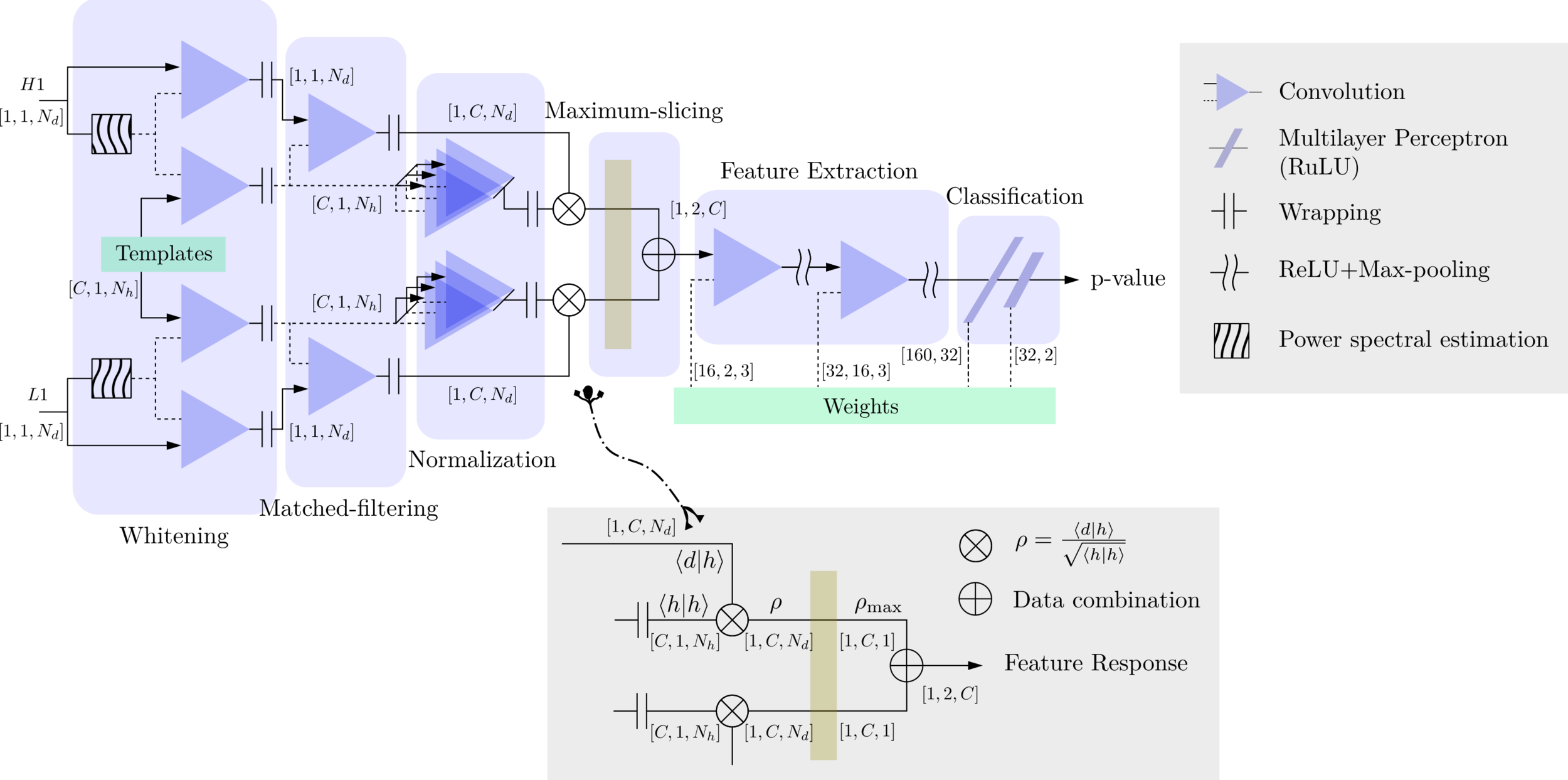
MFCNN
MFCNN
MFCNN
Classification
Feature extraction
Convolutional neural network (ConvNet or CNN)
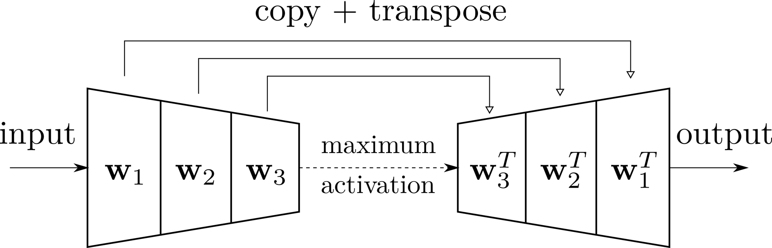
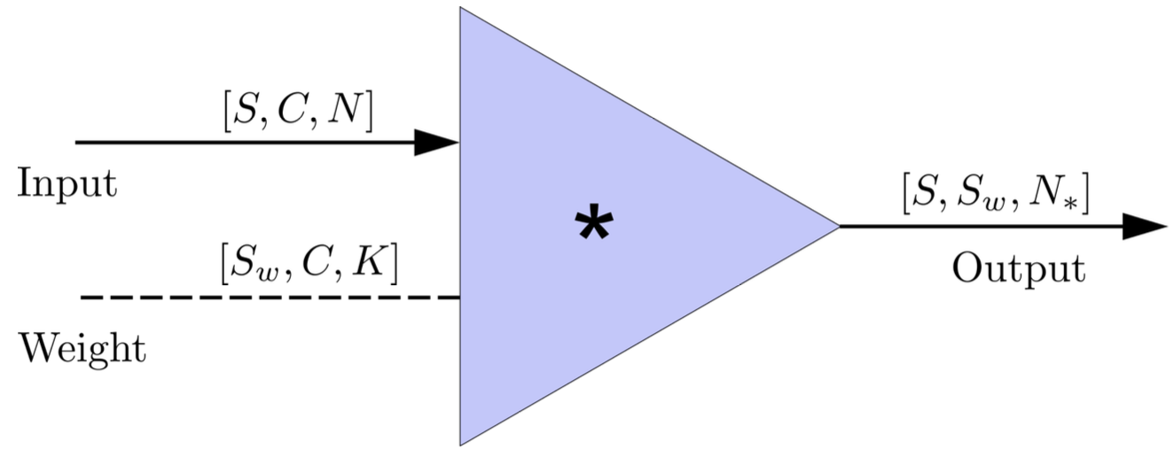
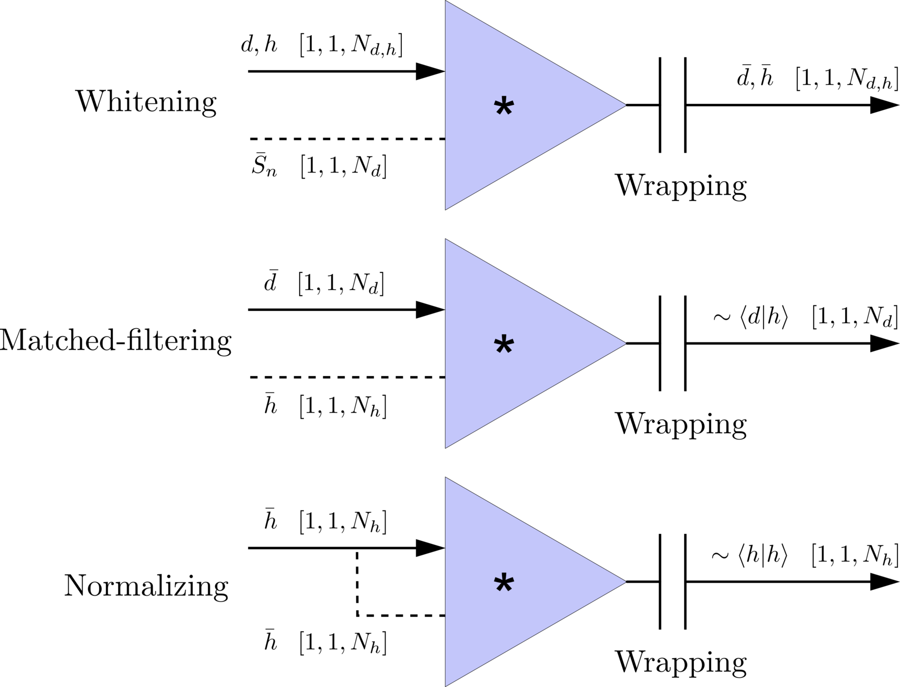
Matched-filtering (cross-correlation with the templates) can be regarded as a convolutional layer with a set of predefined kernels.
>>Is it matched-filtering ?
>>Wait, It can be matched-filtering!
Classification
Feature extraction
Convolutional neural network (ConvNet or CNN)
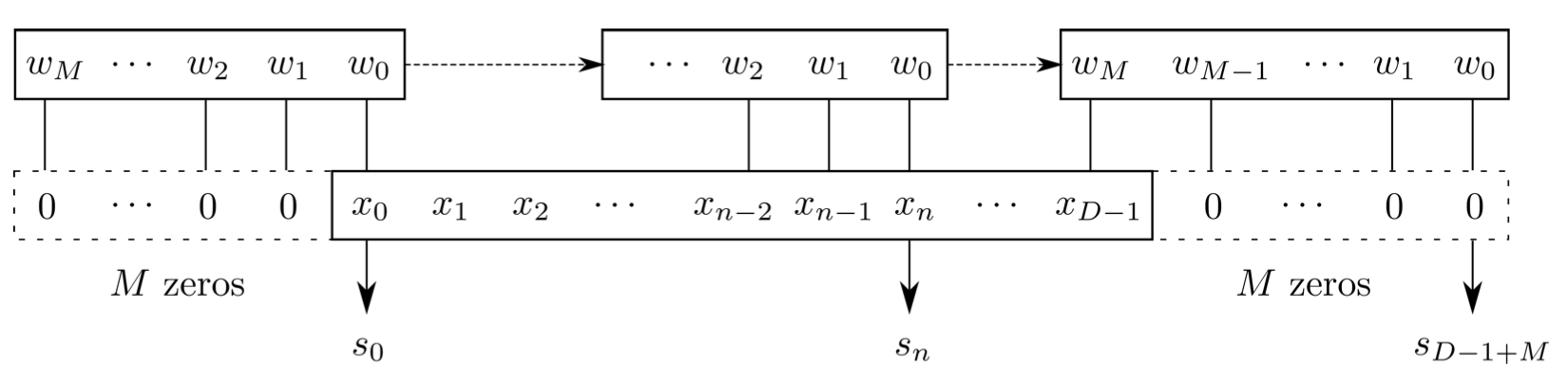
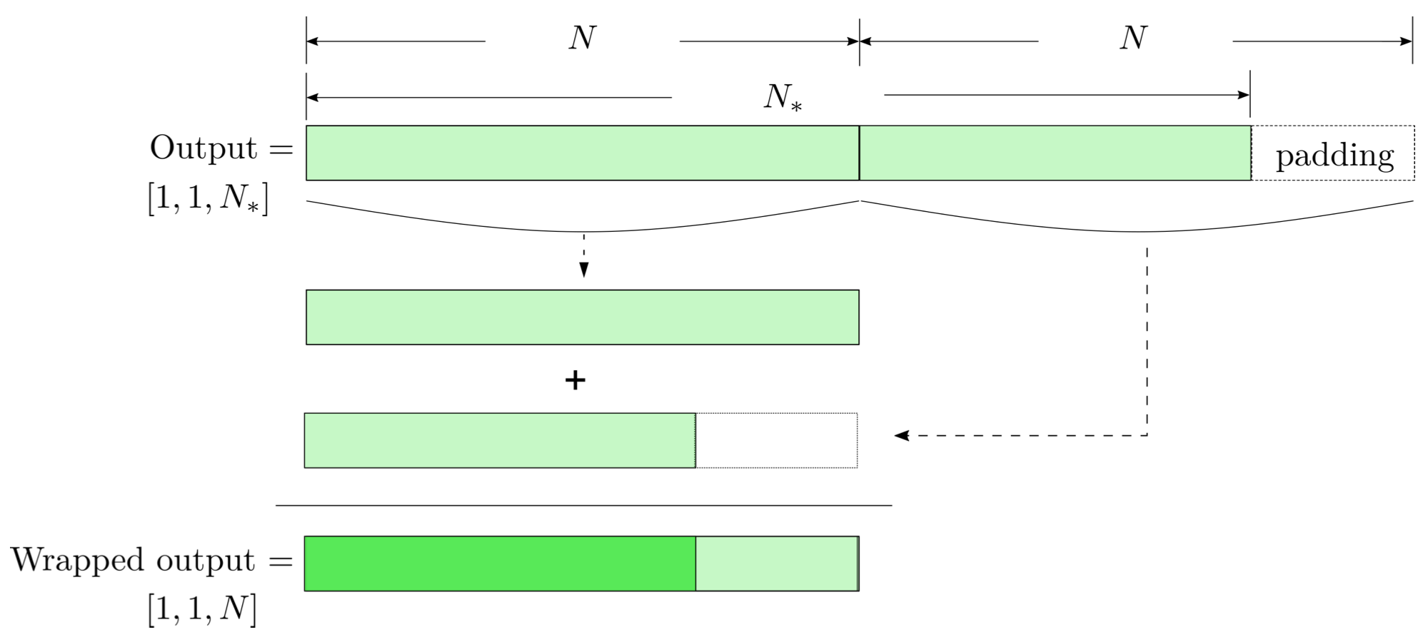
FYI: \(N_\ast = \lfloor(N-K+2P)/S\rfloor+1\)
(A schematic illustration for a unit of convolution layer)
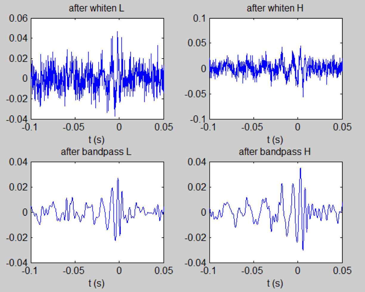
\(S_n(|f|)\) is the one-sided average PSD of \(d(t)\)
(whitening)
where
Time domain
Frequency domain
(normalizing)
(matched-filtering)
\(S_n(|f|)\) is the one-sided average PSD of \(d(t)\)
(whitening)
where
Time domain
Frequency domain
(normalizing)
(matched-filtering)
Deep Learning Framework
modulo-N circular convolution
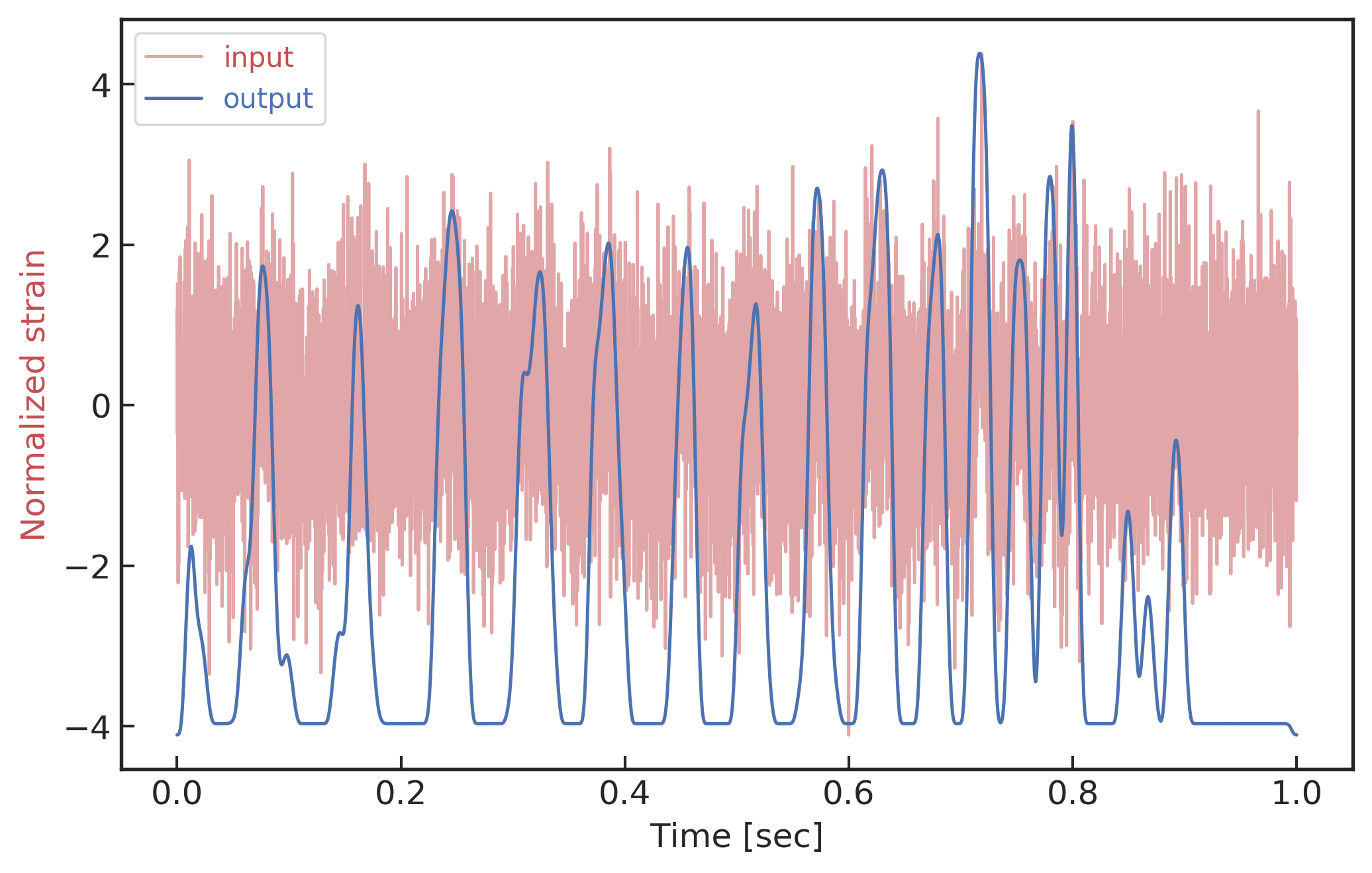
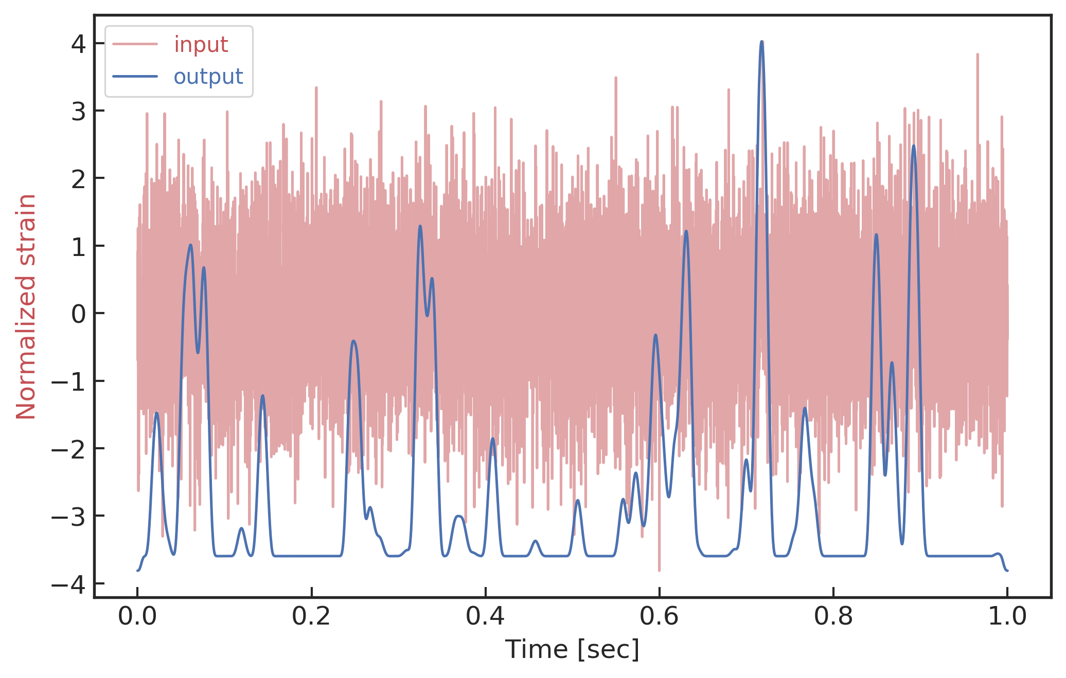
Input
Output
Input
Output
FYI: sampling rate = 4096Hz
| template | waveform (train/test) | |
|---|---|---|
| Number | 35 | 1610 |
| Length (s) | 1 | 5 |
| equal mass |
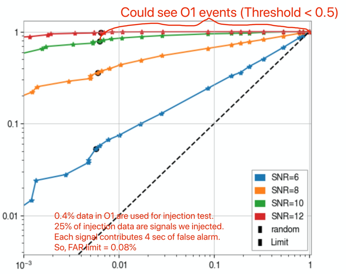
True Positive Rate
False Alarm Rate
input
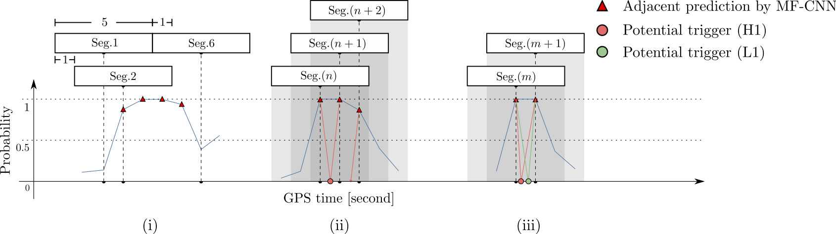
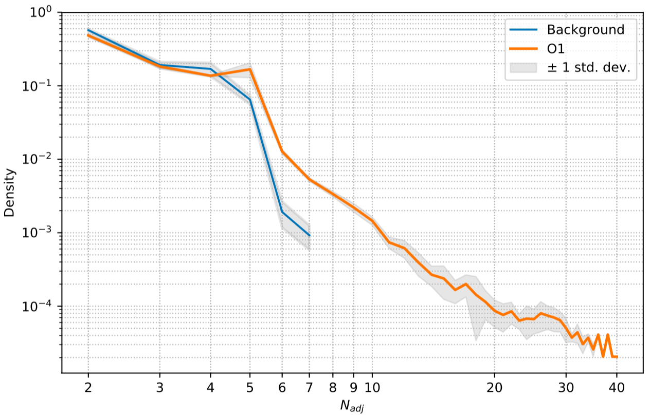
Number of Adjacent prediction
a bump at 5 adjacent predictions
Some benefits from MF-CNN architecture:
Simple configuration for GW data generation and almost no data pre-processing.
Easy parallel deployments, multiple detectors can benefit a lot from this design.
Need to be improved:
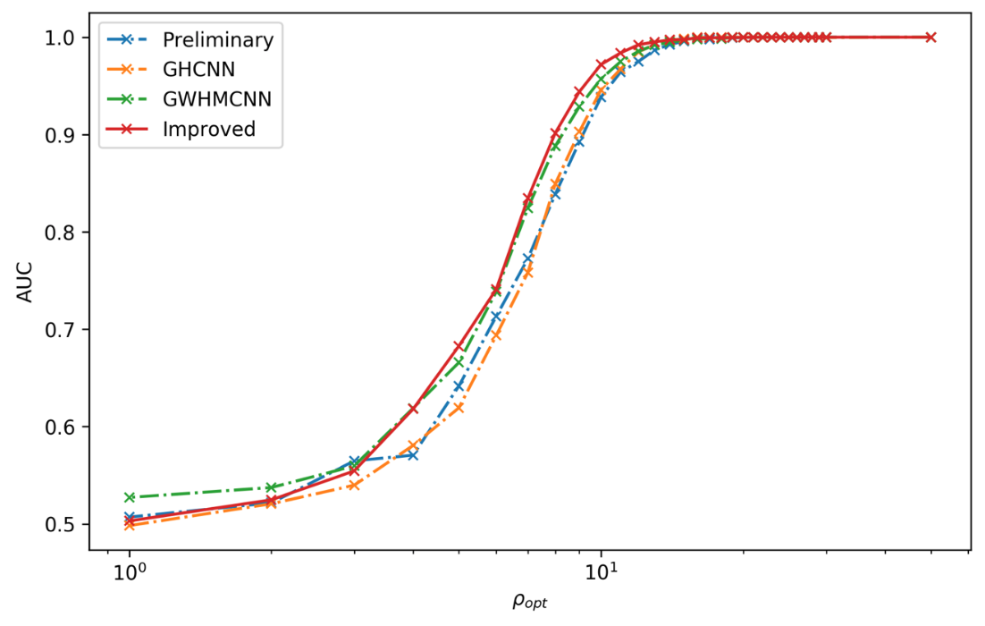
Higher sensitivity
Lower false alarm rate (appropriate metric for estimation)
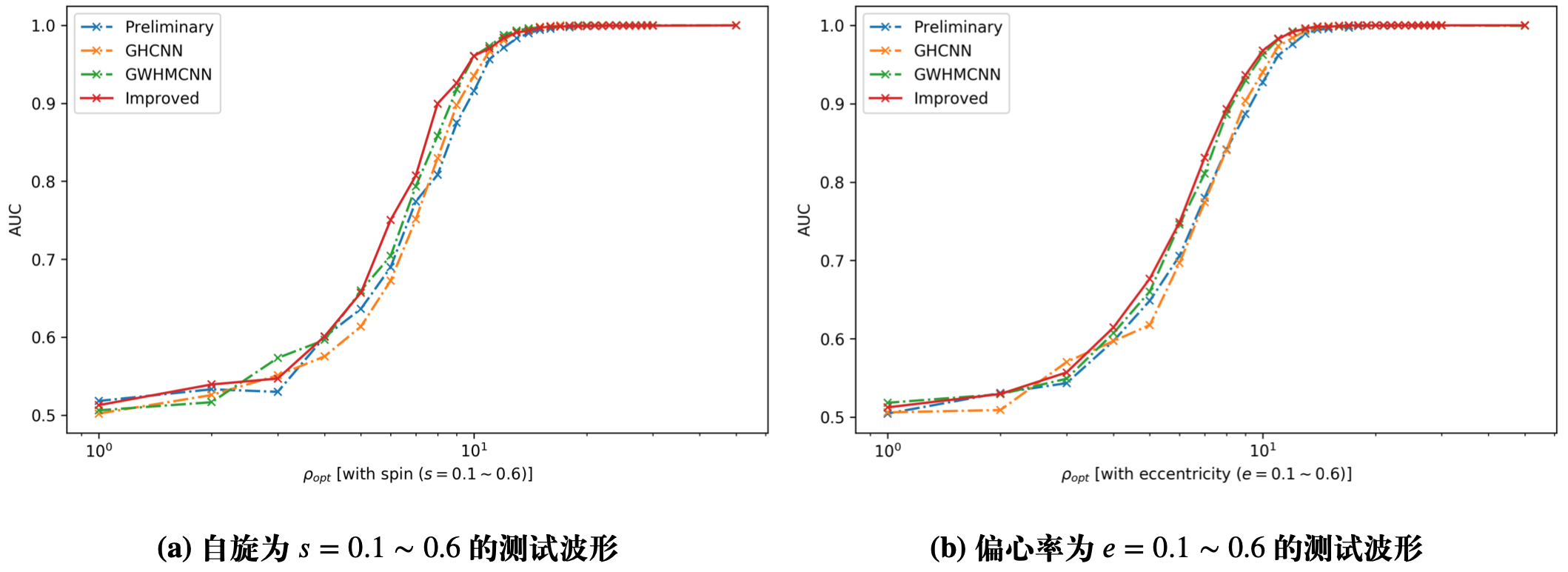
For more GW sources.
Look forward
Parameter estimation (the current “holy grail” of machine learning for GWs.)
GW denoising
"Statistical Learning" / "Theory of Machine Learning" /
...
This slide: https://slides.com/iphysresearch/mf_dl
Some benefits from MF-CNN architecture:
Simple configuration for GW data generation and almost no data pre-processing.
Easy parallel deployments, multiple detectors can benefit a lot from this design.
Need to be improved:
Higher sensitivity
Lower false alarm rate (appropriate metric for estimation)
For more GW sources.
Look forward
Parameter estimation (the current “holy grail” of machine learning for GWs.)
GW denoising
"Statistical Learning" / "Theory of Machine Learning" /
...
for _ in range(num_of_audiences):
    print('Thank you for your attention!')
This slide: https://slides.com/iphysresearch/mf_dl
By He Wang
Webniar


