Efficient Numerical Methods for Nonlinear Model Predictive Control with Applications in Adaptive Cruise Control
Ihno Schrot — Disputationsvortrag — 03. Juli 2025
Ihno Schrot — Efficient Numerical Methods for NMPC with Applications in ACC — Disputationsvortrag — 03. Juli 2025
MOTIVATION
Bildquellen: jcomp, bzw. rawpixel.com, auf Freepik
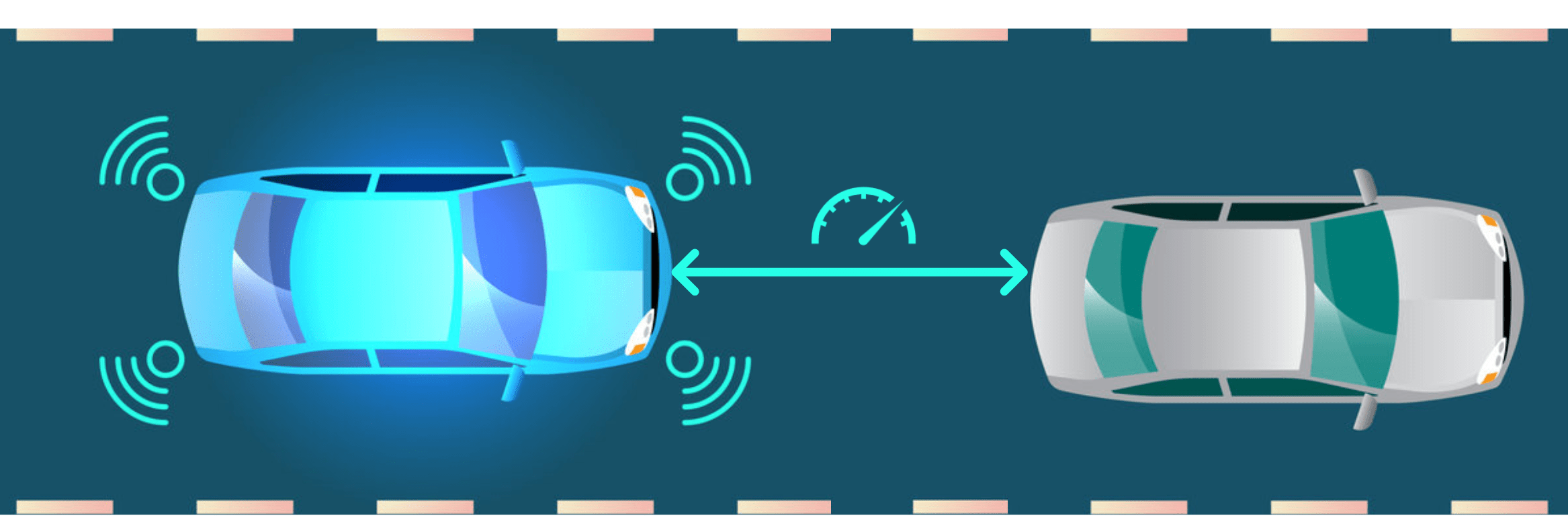
Adaptive Cruise Control (ACC)
- Fahrassistenzsystem
- Tempomat + Abstandshalter

Ecological ACC (EACC)
- Variiert Abstand zum vorigen Fahrzeug (PP0)
- Nutzt Verkehrs- und Streckeninfo \(\rightarrow\) Energiesparen
\(\rightarrow\) Nichtlineare Modellprädiktive Regelung (NMPC)
1/14
- Umgang mit tabellarisierten Daten und externen Einflüssen
- Wenig Rechenleistung auf Onboard-Hardware
Herausforderungen für numerische NMPC Methoden
Ihno Schrot — Efficient Numerical Methods for NMPC with Applications in ACC — Disputationsvortrag — 03. Juli 2025
NICHTLINEARE MODELLPRÄDIKTIVE REGELUNG (NMPC)
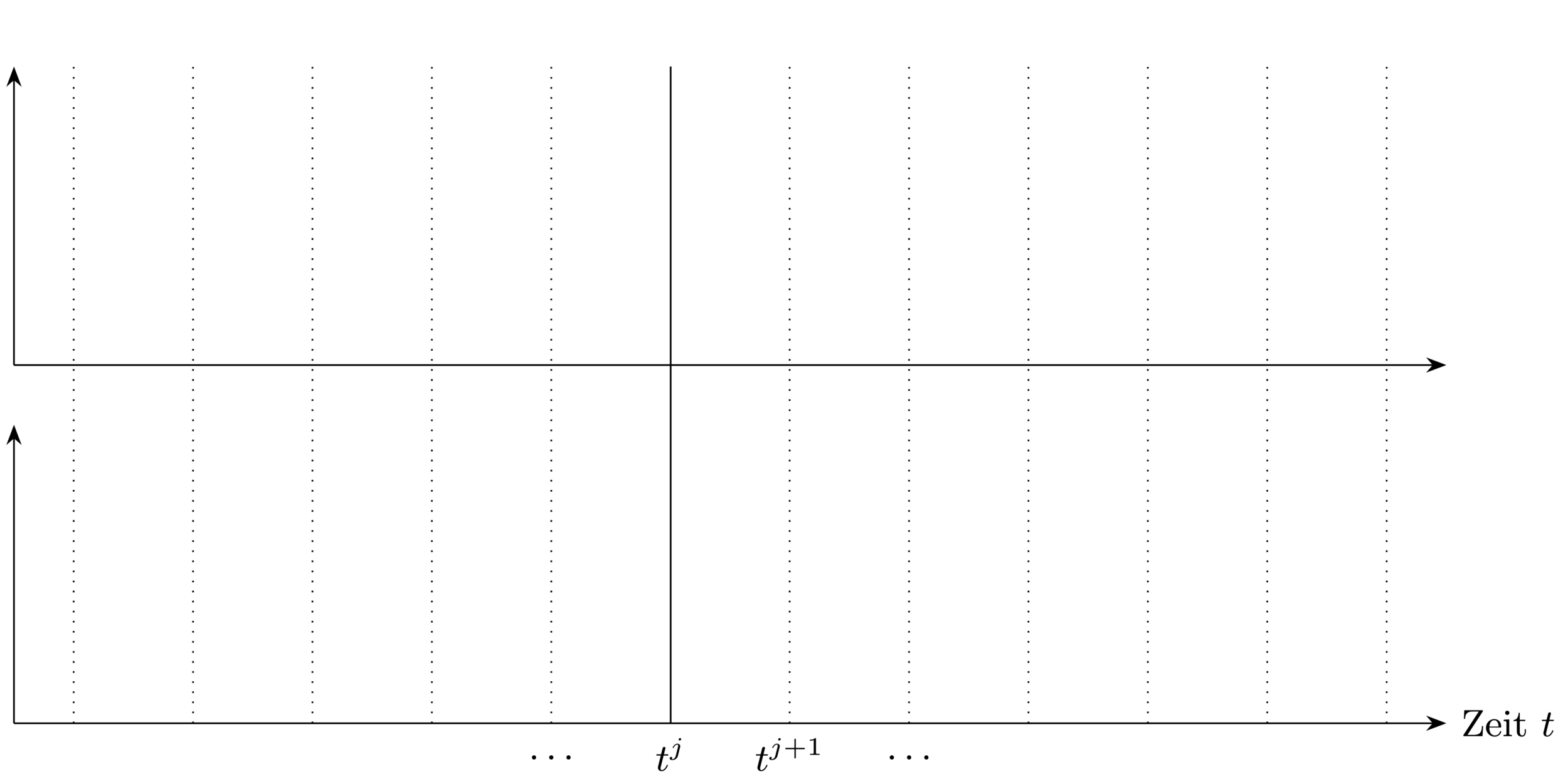
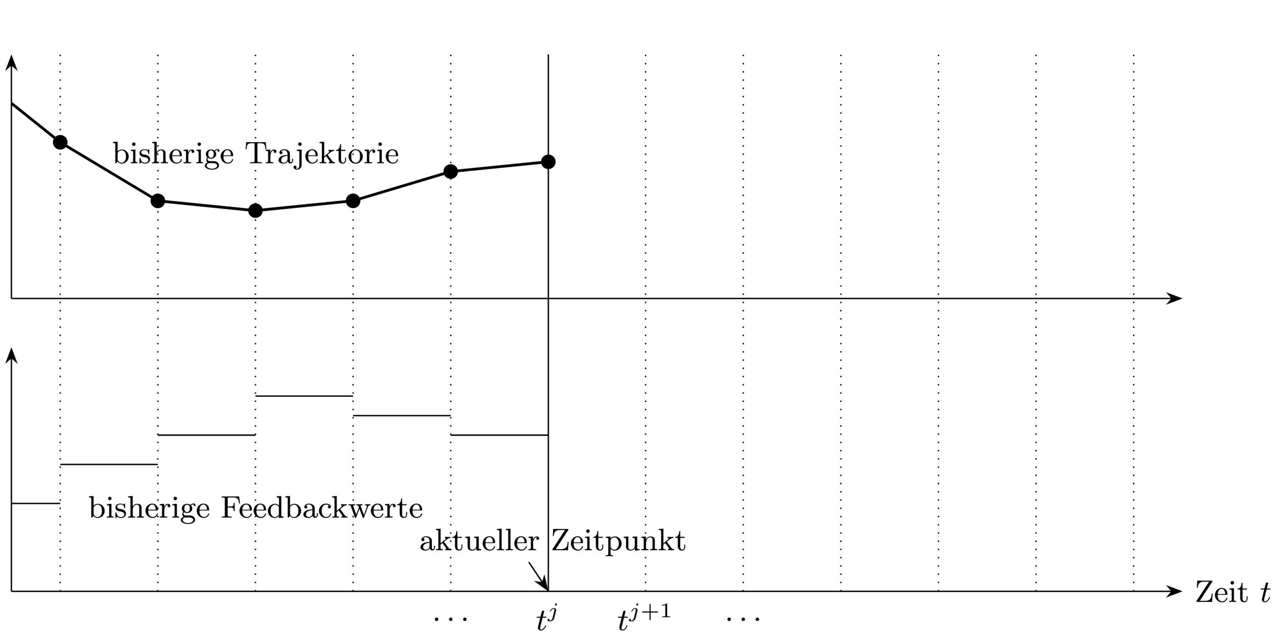
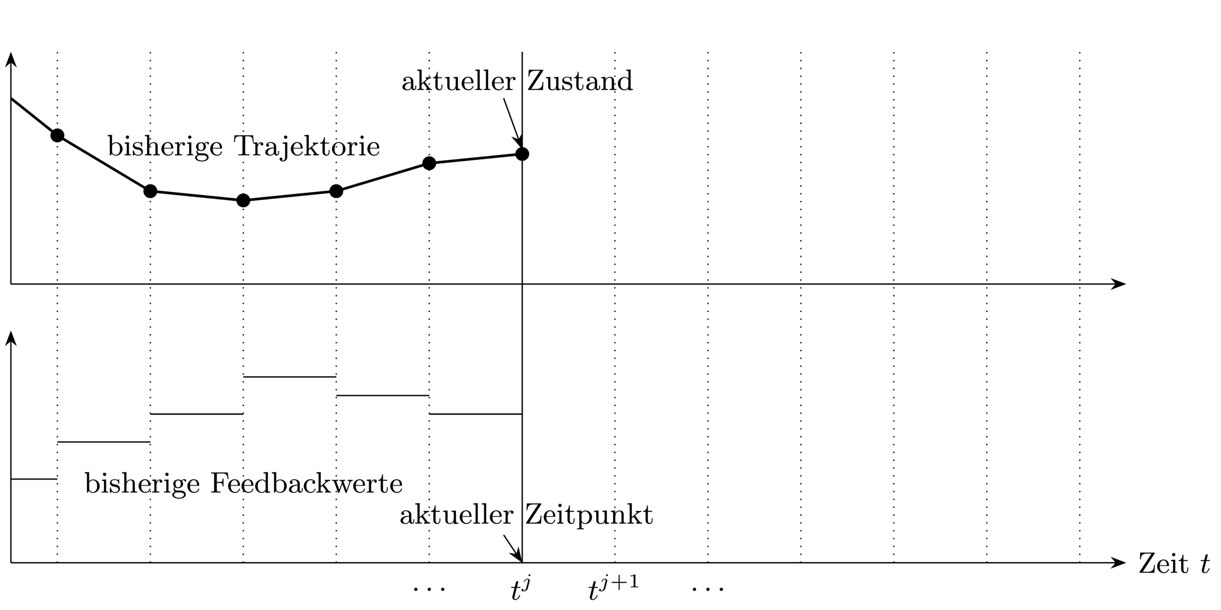
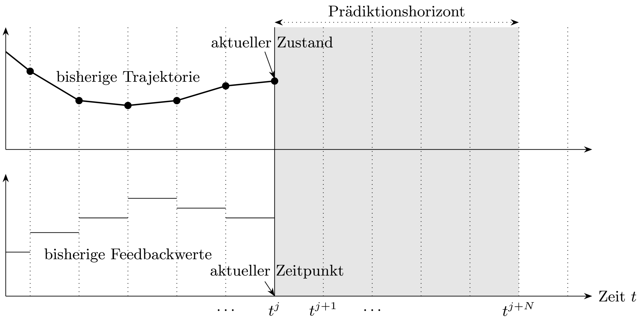
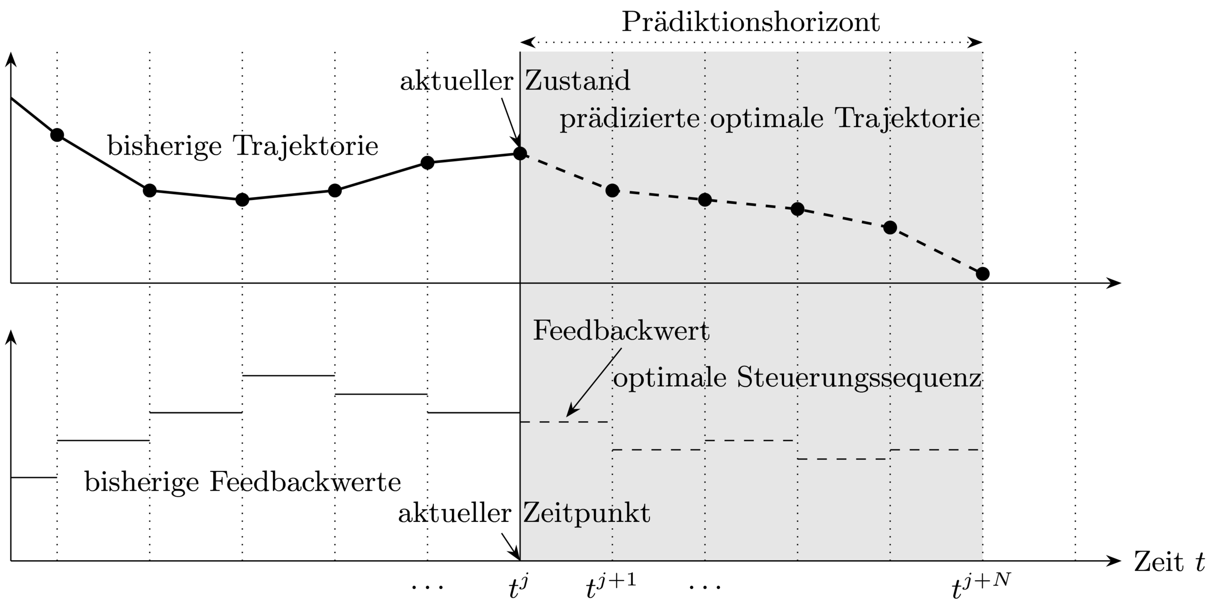
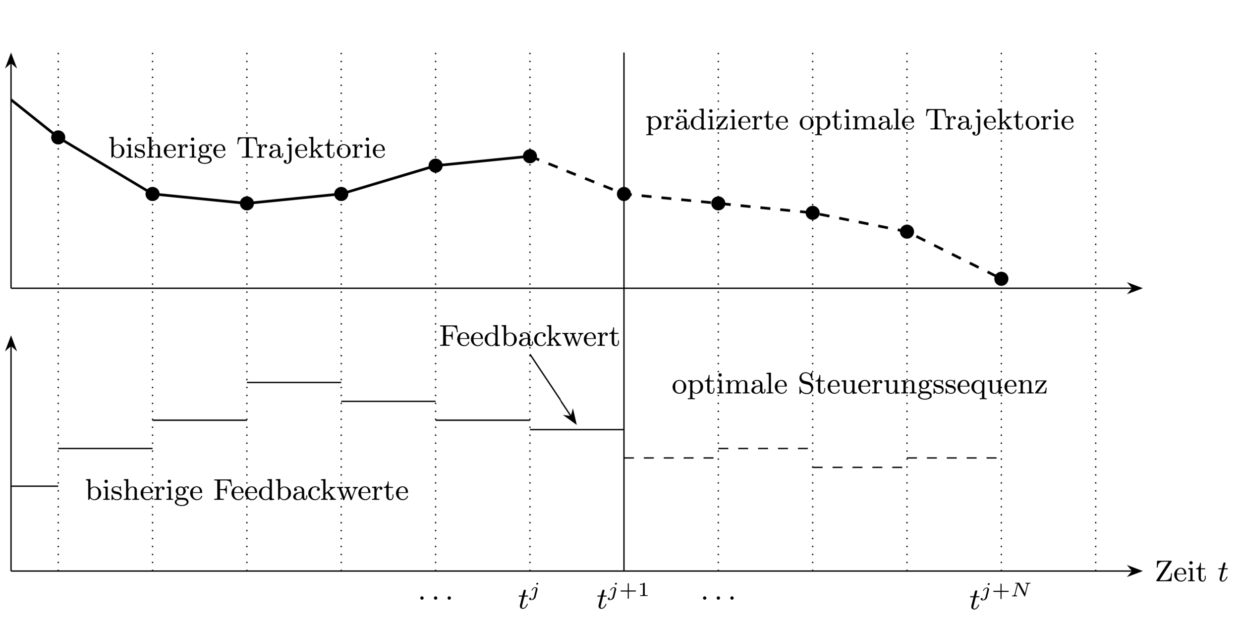
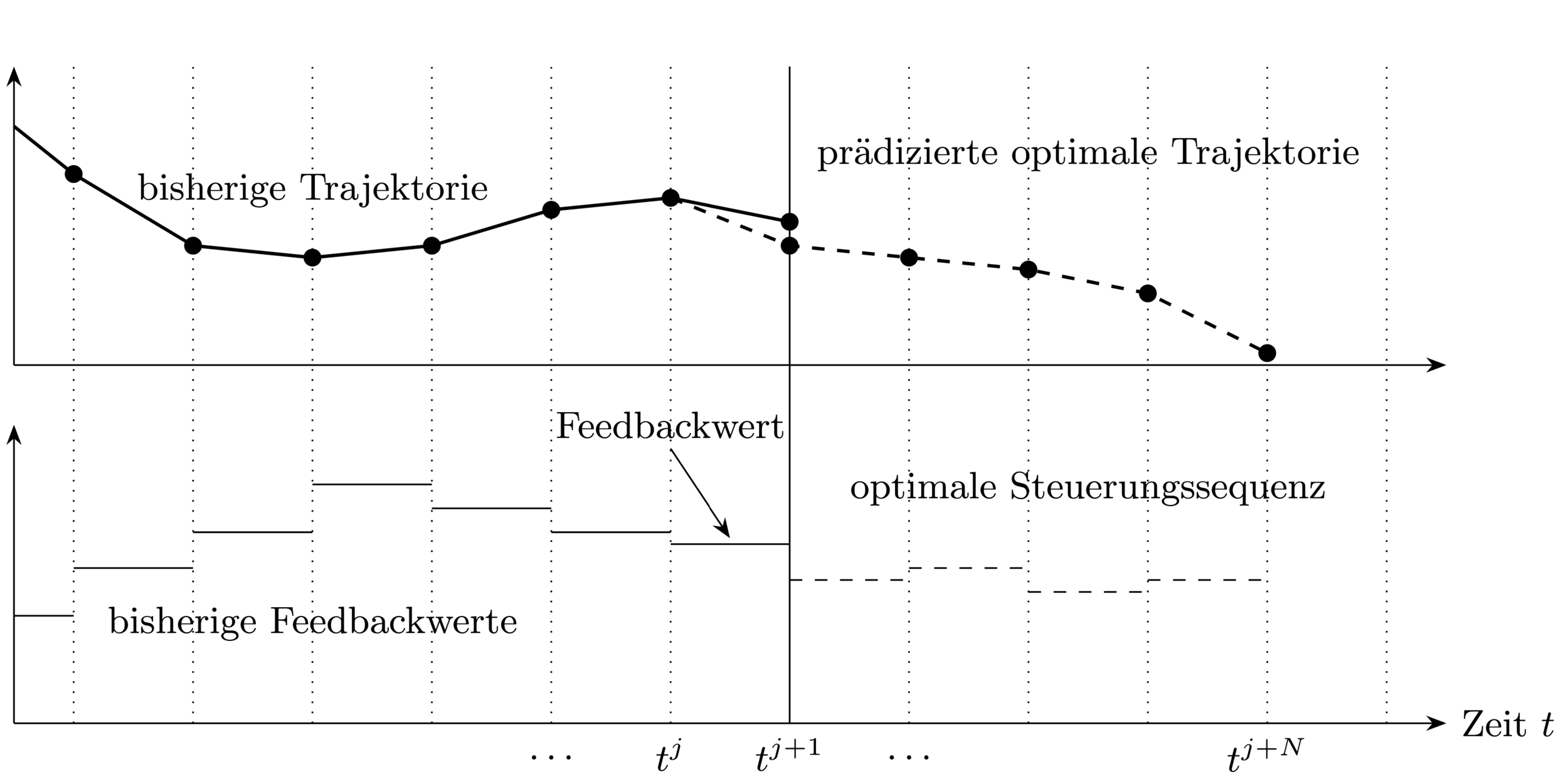
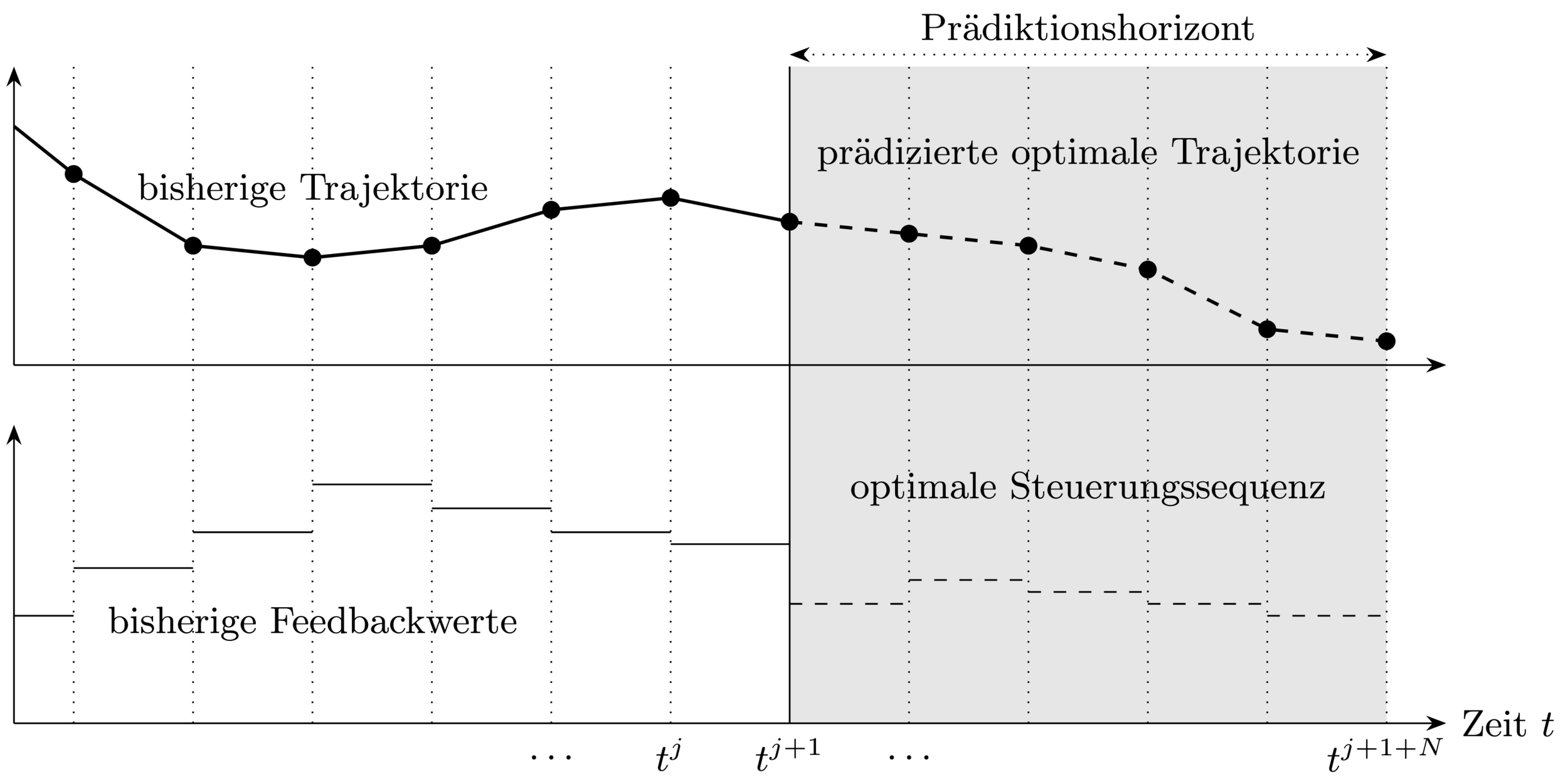
Bei jedem Samplingzeitpunkt:
1. Bestimme aktuellen Zustand
3. Verwende Feedbackwert bis zum nächsten
Samplingzeitpunkt
2. Löse Optimalsteuerungsproblem (OCP) über
Prädiktionshorizont
Closed-loop Steuerungsstrategie \(\rightarrow\) erlaubt auf Störungen zu reagieren
2/14
Ihno Schrot — Efficient Numerical Methods for NMPC with Applications in ACC — Disputationsvortrag — 03. Juli 2025
FRAMEWORK ZUM EFFIZIENTEN LÖSEN VON FOLGEN VON OCPs
\newcommand{\ud}{\mathrm{d}}
\begin{aligned}
&\min_{x(\cdot),u(\cdot)} & \int_{t^j}^{t^j+T} &\Psi\left(x(t),u(t)\right) \ud t +
\Phi\left(x(t^j+T)\right)\\
&\quad\text{s.\,t. }& \dot{x}(t) &= f\left(x(t),u(t)\right),\quad t\in[t^j,t^j+T],\\
&& x(t^j) &= x^j,&&\\
&& 0 &\leq h\left(x(t),u(t)\right),\quad t\in[t^j,t^j+T],\\
&& 0 &= r^{\mathrm{e}} \left(x(t^j),x(t^j+T)\right),\\
&& 0 &\leq r^{\mathrm{i}} \left(x(t^j),x(t^j+T)\right).
\end{aligned}
Systemzustand
und
Steuerung
Systemzustand
und
Steuerung
Laufende und terminale Kosten
Laufende und terminale Kosten
ODE Modell
ODE Modell
Gemischte Zustands- und Steuerungspfadnebenbedingungen
+
Randbedingungen
Modellierung
3/14
Ihno Schrot — Efficient Numerical Methods for NMPC with Applications in ACC — Disputationsvortrag — 03. Juli 2025
FRAMEWORK ZUM EFFIZIENTEN LÖSEN VON FOLGEN VON OCPs
\newcommand{\ud}{\mathrm{d}}
\begin{aligned}
&\min_{x(\cdot),u(\cdot)} & \int_{t^j}^{t^j+T_\mathrm{hor}} &\Psi\left(x(t),u(t)\right) \ud t +
\Phi\left(x(t^j+T_\mathrm{hor})\right)\\
&\quad\text{s.\,t. }& \dot{x}(t) &= f\left(x(t),u(t)\right),\quad t\in[t^j,t^j+T_\mathrm{hor}],\\
&& x(t^j) &= x^j,&&\\
&& 0 &\leq h\left(x(t),u(t)\right),\quad t\in[t^j,t^j+T_\mathrm{hor}],\\
&& 0 &= r^{\mathrm{e}} \left(x(t^j),x(t^j+T_\mathrm{hor})\right),\\
&& 0 &\leq r^{\mathrm{i}} \left(x(t^j),x(t^j+T_\mathrm{hor})\right).
\end{aligned}
\(\infty\) - dimensionales OCP
Modellierung
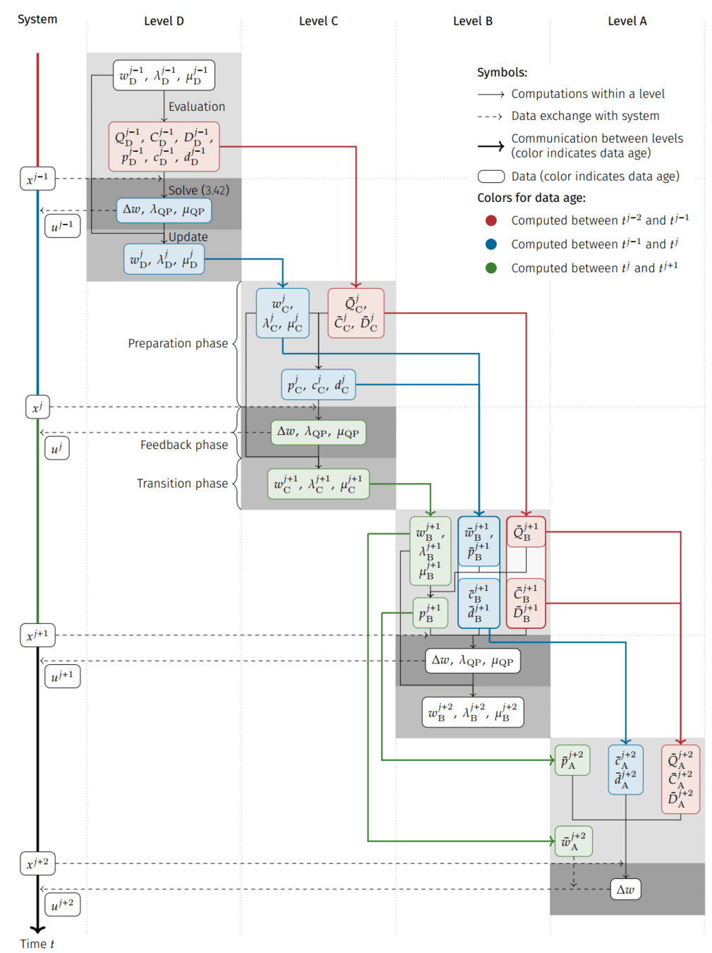
Multi-Level Iterations (MLI)
[Wirsching, 2018]
Real-Time Iterations (RTI)
[Diehl et. al, 2002]
\newcommand{\ud}{\mathrm{d}}
\begin{aligned}
&\min_{\substack{s\in\mathbb{R}^{n_s}\\q\in\mathbb{R}^{n_q}}} & \sum_{m=0}^{N-1} &\Psi_m\left(s_m,q_m\right) +
\Phi\left(s_N\right)\\
&\quad\text{s.\,t. }& 0 &= x\left(\tau_{m+1};s_m,q_m\right)-s_{m+1},\quad m=0,\ldots,N-1,\\
&& 0 &= x^j - s_0,&&\\
&& 0 &\leq h\left(s_m,q_m\right),\quad m=0,\ldots,N-1,\\
&& 0 &= r^{\mathrm{e}} \left(s_0,s_N\right),\\
&& 0 &\leq r^{\mathrm{i}} \left(s_0,s_N\right).
\end{aligned}
Nichtlineares Programm (NLP)
Direct Multiple Shooting (DMS)
[Bock, Plitt 1984]
Meine Beiträge
Theoretische Grundlagen
- [Bock, Plitt, 1984] H. G. Bock and K. J. Plitt. “A Multiple Shooting Algorithm for Direct Solution of Optimal Control Problems”. In: IFAC Proceedings Volumes 17.2 (1984). 9th IFAC World Congress: A Bridge Between Control Science and Technology, Budapest, Hungary, 2-6 July 1984, pp. 1603–1608
- [Diehl et. al., 2002] M. Diehl, H. G. Bock, J. P. Schlöder, R. Findeisen, Z. Nagy, and F. Allgöwer. “Real-time optimization and nonlinear model predictive control of processes governed by differential-algebraic equations”. In: Journal of Process Control 12.4 (2002), pp. 577–585
- [Wirsching, 2018] L. Wirsching. “Multi-level iteration schemes with adaptive level choice for nonlinear model predictive control”. PhD thesis. Heidelberg University, 2018
\newcommand{\ud}{\mathrm{d}}
\begin{aligned}
&\min_{\substack{\Delta s\in\mathbb{R}^{n_s}\\\Delta q\in\mathbb{R}^{n_q}}} & &\frac{1}{2}\begin{pmatrix}\Delta s \\ \Delta q\end{pmatrix}^T\begin{pmatrix}B^{ss} & B^{sq} \\ B^{qs} & B^{qq}\end{pmatrix}\begin{pmatrix}\Delta s \\ \Delta q\end{pmatrix} + \begin{pmatrix}b^s\\b^q\end{pmatrix}^T\begin{pmatrix}\Delta s \\ \Delta q\end{pmatrix}\\
&\quad\text{s.\,t. }& 0 &= S_m^s\Delta s_m + S_m^q\Delta q_m - \Delta s_{m+1},\quad m=0,\ldots,M-1,\\
&& 0 &= x^j - s_0 - \Delta s_0,&&\\
&& 0 &\leq H_m^s\Delta s_m + H_m^q\Delta q_m + h_m,\quad m=0,\ldots,M-1,\\
&& 0 &= R_{s_0}^\mathrm{e}\Delta s_0 + R_{s_M}^\mathrm{e}\Delta s_M + r^\mathrm{e},\\
&& 0 &\leq R_{s_0}^\mathrm{i}\Delta s_0 + R_{s_M}^\mathrm{i}\Delta s_M + r^\mathrm{i}.
\end{aligned}
Quadratisches Programm (QP)
Zugeschnittenes SQP-Verfahren
3/14
Ihno Schrot — Efficient Numerical Methods for NMPC with Applications in ACC — Disputationsvortrag — 03. Juli 2025
MEINE BEITRÄGE
1.
2.
3.
4.
ANWENDUNG:
EACC
-
Realistisches Testproblem mit realen Kennfeldern und Fahrdaten
-
Erfolgreiche numerische Tests

STABILITÄT BEI INEXAKTEM NMPC
-
OCP semilinear parabolischer PDEs
-
Beweis asymptotischer Stabilität der System-Optimierer-Dynamik
FORM-ERHALTENDE
INTERPOLATION
-
Klassifikation im multivariaten Fall
-
Methode zur multivariaten, form-erhaltenden, glatten Interpolation
-
Berücksichtigung externer Einflüsse bei DMS, RTI und MLI
-
Angepasste Condensing-Strategien
EXTERNE EINFLÜSSE

-
Szenariobasiertes Online-Feedback
-
Online-Aufwand: Matrix-Vektor-Multiplikation oder Lösen eines QPs

SensEIS
FEEDBACK
4/14
Ihno Schrot — Efficient Numerical Methods for NMPC with Applications in ACC — Disputationsvortrag — 03. Juli 2025
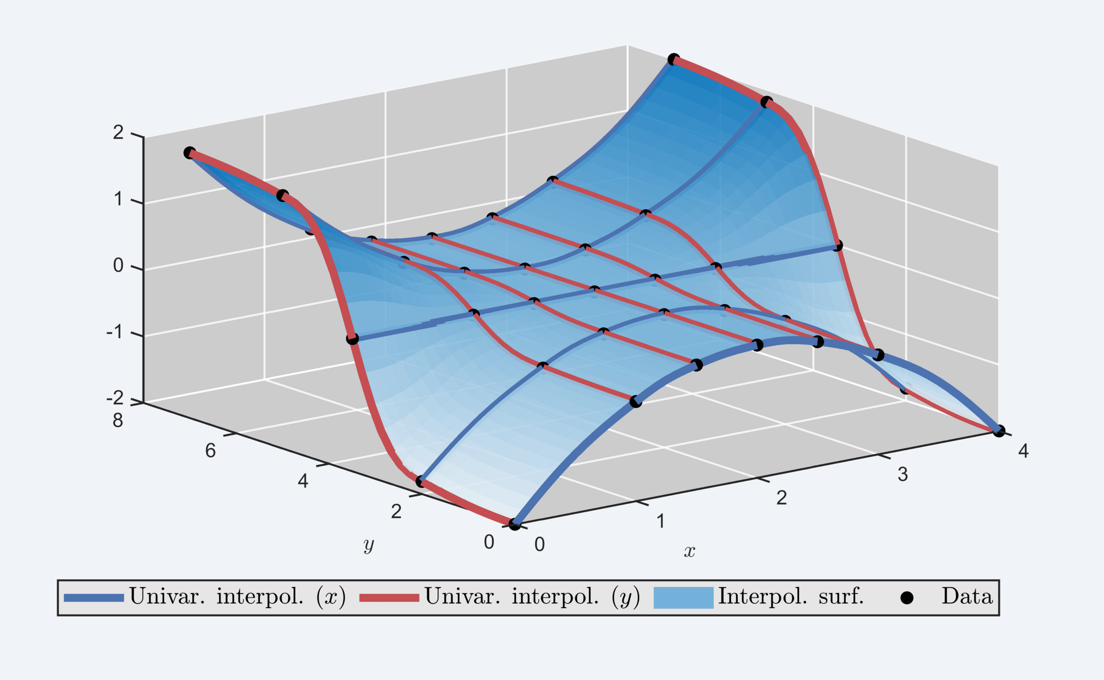
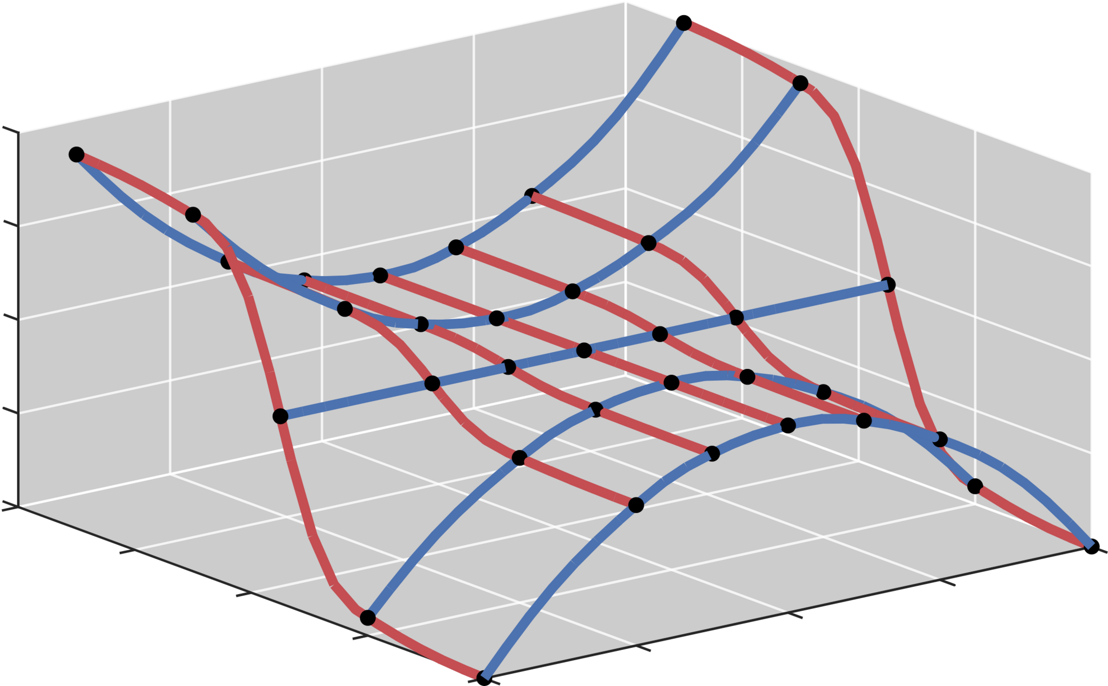
FORMERHALTENDE GLATTE INTERPOLATION
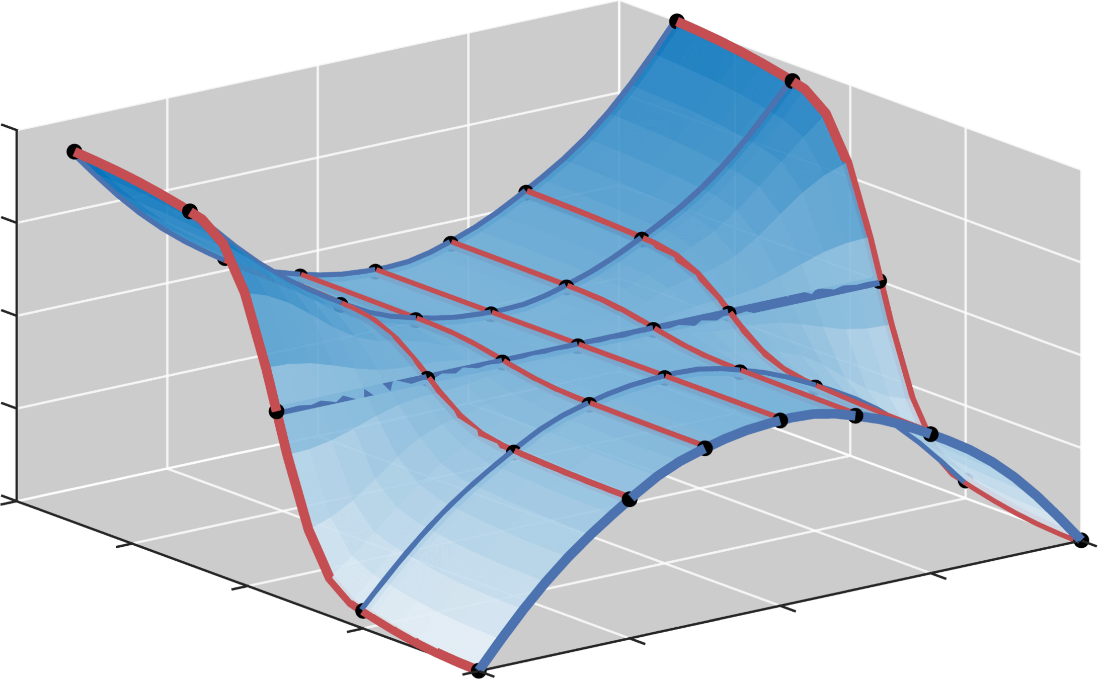
BESONDERHEITEN MEINER METHODE:
- Modularität: Univariate Methode frei wählbar
- Erbt Glattheit, Formerhaltung und Lokalität der univariaten Methode
- [Costantini, 1988] P. Costantini. “An algorithm for computing shape-preserving interpolating splines of arbitrary degree”. In: Journal of Computational and Applied Mathematics 22.1 (1988), pp. 89–136
- [Coons, 1967] S. A. Coons. Surfaces for computer-aided design of space forms. Tech. rep. Project MAC-TR 41. USA: MIT, 1967
MEINE METHODE:
Schritt 1: Formerhaltende glatte univariate Interpolation entlang der Gitterlinien, bspw. mit [Costantini, 1988]
Schritt 2: Gewichtung der univariaten Interpolation durch höherdimensionale Erweiterung von Coons' Patches [Coons, 1967]
THEMA: Interpolation multivariater tabellarisierter Daten (Kennfelder)
HERAUSFORDERUNGEN:
- Aus Modellierung: Formerhaltung (Monotonie, Konvexität u. ä.)
- Aus Optimierung: Glatte Interpolation (sonst Undifferenzierbarkeiten in OCP!)
5/14
Ihno Schrot — Efficient Numerical Methods for NMPC with Applications in ACC — Disputationsvortrag — 03. Juli 2025
MEINE BEITRÄGE
2.
ANWENDUNG:
EACC
-
Realistisches Testproblem mit realen Kennfeldern und Fahrdaten
-
Erfolgreiche numerische Tests
STABILITÄT BEI INEXAKTEM NMPC
-
OCP semilinear parabolischer PDEs
-
Beweis asymptotischer Stabilität der System-Optimierer-Dynamik
FORM-ERHALTENDE
INTERPOLATION
-
Klassifikation im multivariaten Fall
-
Methode zur multivariaten, form-erhaltenden, glatten Interpolation
-
Berücksichtigung externer Einflüsse bei DMS, RTI und MLI
-
Angepasste Condensing-Strategien
EXTERNE EINFLÜSSE
-
Szenariobasiertes Online-Feedback
-
Online-Aufwand: Matrix-Vektor-Multiplikation oder Lösen eines QPs
SensEIS
FEEDBACK
6/14
Ihno Schrot — Efficient Numerical Methods for NMPC with Applications in ACC — Disputationsvortrag — 03. Juli 2025
SensEIS FEEDBACK
MEINE METHODE:
...

Löse
OCP
Löse
OCP
Löse
OCP
THEMA: Schnelles Online-Feedback
VARIANTEN MEINER METHODE:
- Feedbackmatrix: Nur Matrix-Vektor-Multiplikation als Online-Aufwand
- Feedbackgenerierendes QP: Berücksichtigt Active-Set-Wechsel
- Kombinierbar mit MLI oder eigenständige Methode
HERAUSFORDERUNGEN:
- Aus Anwendung: Möglichst geringer Online-Rechenwaufwand
- Aus Optimierung: Kombinierbar mit MLI
Optimale Lösung &
Feedbackoperator
Optimale Lösung &
Feedbackoperator
Optimale Lösung &
Feedbackoperator
Offline-Phase
Online-Phase

Neue
Steuerung
Feedbackoperator
aus Szenario
Aktueller Systemzustand
Optimale Lösung aus Szenario
7/14
Ihno Schrot — Efficient Numerical Methods for NMPC with Applications in ACC — Disputationsvortrag — 03. Juli 2025
SensEIS FEEDBACK - FEEDBACKGENERIERENDES QP
QP IM ZUGESCHNITTENEN SQP-VERFAHREN
NEUE KOMPONENTEN
\newcommand{\ud}{\mathrm{d}}
% \definecolor{hlc}{HTML}{AA947B}
\begin{aligned}
&\quad\min_{\substack{\Delta s\in\mathbb{R}^{n_s}\\\Delta q\in\mathbb{R}^{n_q}}} \frac{1}{2}\begin{pmatrix}\Delta s \\ \Delta q\end{pmatrix}^T\begin{pmatrix}B^{ss} & B^{sq} \\ B^{qs} & B^{qq}\end{pmatrix}\begin{pmatrix}\Delta s \\ \Delta q\end{pmatrix} \hspace{0.25cm} + \begin{pmatrix}b^s\\b^q\end{pmatrix}^T\begin{pmatrix}\Delta s \\ \Delta q\end{pmatrix} \hspace{0.4cm} + \begin{pmatrix}\Delta x^j \\ \Delta \rho^j \\ \Delta v^j\end{pmatrix}^T\begin{pmatrix}B^{\hat{x}s} & B^{\hat{x}q} \\ B^{\rho s} & B^{\rho q} \\ B^{v s} & B^{v q}\end{pmatrix}\begin{pmatrix}\Delta s \\ \Delta q\end{pmatrix}\\[2em]
& \left\{ \quad\text{s.\,t. }\quad
\begin{aligned}
& 0 = -\Delta s_0 &&&& & \hspace{0.25cm} & +\Delta x^j &&&&\\
& 0 = S_m^s\Delta s_m - \Delta s_{m+1} &&+ S_m^q\Delta q_m && &&&& + S_m^\rho\Delta\rho^j &&+ S_m^v\Delta v^j,\\
& 0 \leq H_m^s\Delta s_m &&+ H_m^q\Delta q_m &&+ h_m &&&& + H_m^\rho\Delta\rho^j &&+ H_m^v\Delta v^j,\\
& 0 = R_{s_0}^\mathrm{e}\Delta s_0 + R_{s_M}^\mathrm{e}\Delta s_M &&&& &&&&+ R^{\mathrm{e}}_{\rho}\Delta\rho^j &&+ R^{\mathrm{e}}_{v_0}\Delta v_0^j + R^{\mathrm{e}}_{v_M}\Delta v_M^j,\\
& 0 \leq R_{s_0}^\mathrm{i}\Delta s_0 + R_{s_M}^\mathrm{i}\Delta s_M &&&&+ r^\mathrm{i} &&&&+ R^{\mathrm{i}}_{\rho}\Delta\rho^j &&+ R^{\mathrm{i}}_{v_0}\Delta v_0^j + R^{\mathrm{i}}_{v_M}\Delta v_M^j.
\end{aligned}
\right.
\end{aligned}
Resi-duen
Linearisierung bzgl.
Zuständen u. Steuerung
Hesse-Matrix bzgl.
Zuständen und Steuerung
Gradient bzgl.
Zuständen und Steuerung
Lin. bzgl.
Parametern
Lin. bzgl. aktuellem Zustand
Linearisierung bzgl.
externen Einflüssen
Hesse-Matrix bzgl. aktuellem Zustand,
Parametern und externen Einflüssen dann Zuständen und Steuerungen
8/14
Variablen:
Zustände und Steuerungen
Linearisiert und ausgewertet in Szenario-lösung
Ihno Schrot — Efficient Numerical Methods for NMPC with Applications in ACC — Disputationsvortrag — 03. Juli 2025
SensEIS FEEDBACK - FEEDBACKGENERIERENDES QP
QP IM ZUGESCHNITTENEN SQP-VERFAHREN
NEUE KOMPONENTEN
Variablen:
Zustände und Steuerungen
\newcommand{\ud}{\mathrm{d}}
% \definecolor{hlc}{HTML}{AA947B}
\begin{aligned}
&\quad\min_{\substack{\Delta s\in\mathbb{R}^{n_s}\\\Delta q\in\mathbb{R}^{n_q}}} \frac{1}{2}\begin{pmatrix}\Delta s \\ \Delta q\end{pmatrix}^T\begin{pmatrix}B^{ss} & B^{sq} \\ B^{qs} & B^{qq}\end{pmatrix}\begin{pmatrix}\Delta s \\ \Delta q\end{pmatrix} \hspace{0.25cm} + \begin{pmatrix}b^s\\b^q\end{pmatrix}^T\begin{pmatrix}\Delta s \\ \Delta q\end{pmatrix} \hspace{0.4cm} + \begin{pmatrix}\Delta x^j \\ \Delta \rho^j \\ \Delta v^j\end{pmatrix}^T\begin{pmatrix}B^{\hat{x}s} & B^{\hat{x}q} \\ B^{\rho s} & B^{\rho q} \\ B^{v s} & B^{v q}\end{pmatrix}\begin{pmatrix}\Delta s \\ \Delta q\end{pmatrix}\\[2em]
& \left\{ \quad\text{s.\,t. }\quad
\begin{aligned}
& 0 = -\Delta s_0 &&&& & \hspace{0.25cm} & +\Delta x^j &&&&\\
& 0 = S_m^s\Delta s_m - \Delta s_{m+1} &&+ S_m^q\Delta q_m && &&&& + S_m^\rho\Delta\rho^j &&+ S_m^v\Delta v^j,\\
& 0 \leq H_m^s\Delta s_m &&+ H_m^q\Delta q_m &&+ h_m &&&& + H_m^\rho\Delta\rho^j &&+ H_m^v\Delta v^j,\\
& 0 = R_{s_0}^\mathrm{e}\Delta s_0 + R_{s_M}^\mathrm{e}\Delta s_M &&&& &&&&+ R^{\mathrm{e}}_{\rho}\Delta\rho^j &&+ R^{\mathrm{e}}_{v_0}\Delta v_0^j + R^{\mathrm{e}}_{v_M}\Delta v_M^j,\\
& 0 \leq R_{s_0}^\mathrm{i}\Delta s_0 + R_{s_M}^\mathrm{i}\Delta s_M &&&&+ r^\mathrm{i} &&&&+ R^{\mathrm{i}}_{\rho}\Delta\rho^j &&+ R^{\mathrm{i}}_{v_0}\Delta v_0^j + R^{\mathrm{i}}_{v_M}\Delta v_M^j.
\end{aligned}
\right.
\end{aligned}
Linearisiert und ausgewertet in Szenario-lösung
Lineare Approximation der Residuuen bzgl.
aktuellem Zustand, Parametern und externen Einflüssen
8/14
Ihno Schrot — Efficient Numerical Methods for NMPC with Applications in ACC — Disputationsvortrag — 03. Juli 2025
MEINE BEITRÄGE
3.
ANWENDUNG:
EACC
-
Realistisches Testproblem mit realen Kennfeldern und Fahrdaten
-
Erfolgreiche numerische Tests
STABILITÄT BEI INEXAKTEM NMPC
-
OCP semilinear parabolischer PDEs
-
Beweis asymptotischer Stabilität der System-Optimierer-Dynamik
FORM-ERHALTENDE
INTERPOLATION
-
Klassifikation im multivariaten Fall
-
Methode zur multivariaten, form-erhaltenden, glatten Interpolation
-
Berücksichtigung externer Einflüsse bei DMS, RTI und MLI
-
Angepasste Condensing-Strategien
EXTERNE EINFLÜSSE
-
Szenariobasiertes Online-Feedback
-
Online-Aufwand: Matrix-Vektor-Multiplikation oder Lösen eines QPs
SensEIS
FEEDBACK
9/14
Ihno Schrot — Efficient Numerical Methods for NMPC with Applications in ACC — Disputationsvortrag — 03. Juli 2025
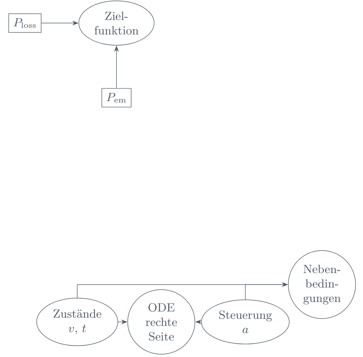
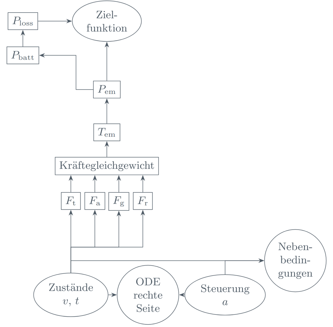
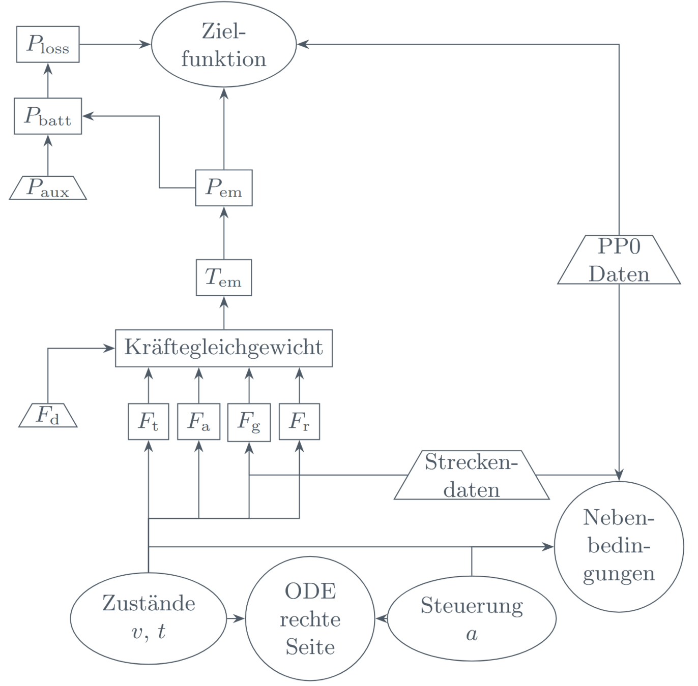
ECOLOGICAL ADAPTIVE CRUISE CONTROL (EACC)
MEINE REALISTISCHE EACC FORMULIERUNG:
-
Freie Variable: Strecke \(s\)
-
Zustände: Geschwindigkeit \(v\) und Zeit \(t\)
-
Steuerung: Beschleunigung \(a\)
\newcommand{\ud}{\mathrm{d}}
\begin{aligned}
&\min_{v(\cdot),\,t(\cdot),\,a(\cdot)} && \int_{s^j}^{s^j+S}\left[ w_0 P_\mathrm{em} + w_1 P_\mathrm{loss} + \sum_{i=1}^{k}w_{i+1}\Psi_i^\mathrm{c}\right]\ud s\\[1.35em]
&\quad\text{s.\,t. }&&
\begin{aligned}
\begin{pmatrix}v'(s)\\t'(s) \end{pmatrix} &= \frac{1}{v(s)} \begin{pmatrix}a(s) \\ 1 \end{pmatrix},&& s\in[s^j,s^j+S],\\
\begin{pmatrix}v(s^j)\\t(s^j) \end{pmatrix} &= \begin{pmatrix} v^j\\t^j\end{pmatrix},&&\\[1.05em]
a_\mathrm{min} &\leq a(s) \leq a_\mathrm{max},&& s\in[s^j,s^j+S],\\
0 & < v(s) \leq v_\mathrm{max}(s),&& s\in[s^j,s^j+S],\\
0 &\leq t(s) - t_\mathrm{PP0}(s) -\Delta t_\mathrm{min},&& s\in[s^j,s^j+S].
\end{aligned}
\end{aligned}
Energieverbrauch und Komfortaspekte
Beschleunigungs-, und Geschwindigkeitsschranken
und Sicherheitsabstand
Energieverbrauch und Komfortaspekte
Beschleunigungs-, und Geschwindigkeitsschranken
und Sicherheitsabstand
10/14
Ihno Schrot — Efficient Numerical Methods for NMPC with Applications in ACC — Disputationsvortrag — 03. Juli 2025
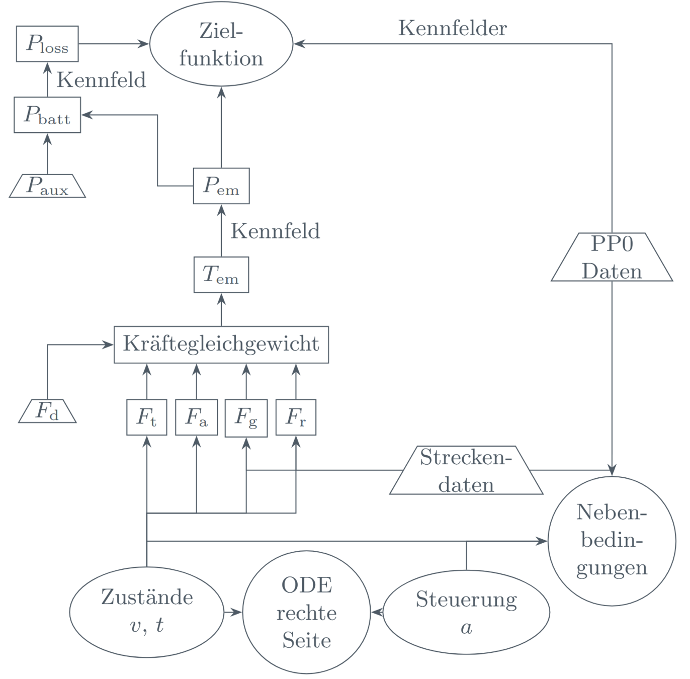
ECOLOGICAL ADAPTIVE CRUISE CONTROL (EACC) — RESULTATE
MEIN TESTSETUP:
-
Echtdaten einer Fahrt von 34,5km in Stuttgart
-
Reale Kennfelder vom Industriepartner
-
Interpolation der Kennfelder mit meiner neuen Methode
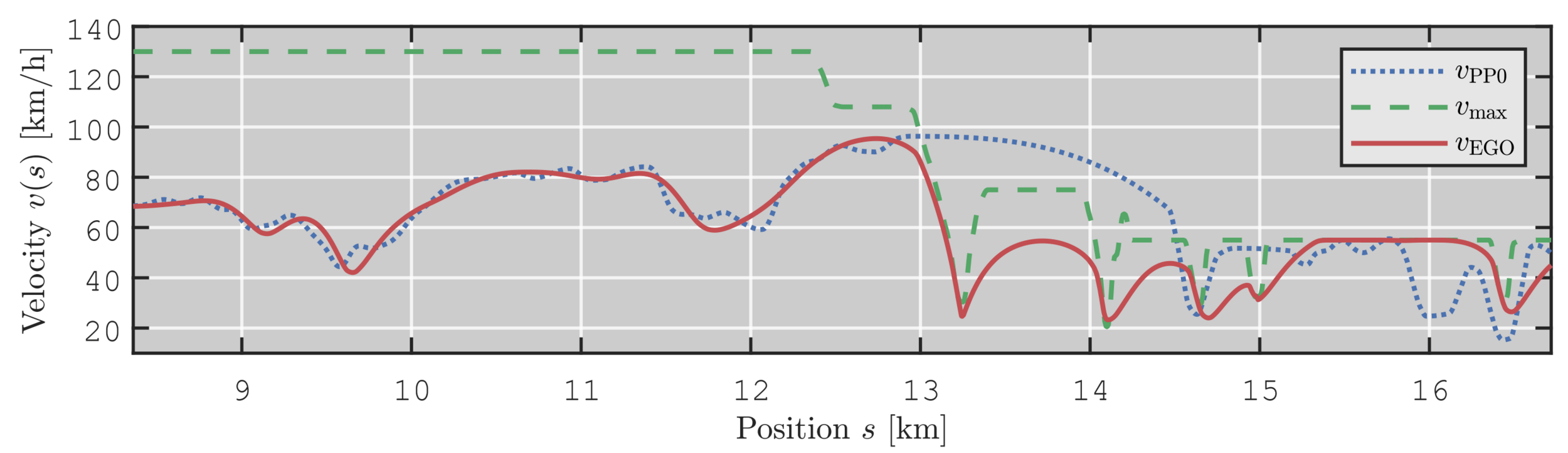
ENERGIEEINSPARUNGEN
- Standard MLI: 3,4%
- MLI mit externen Einflüssen: 4,3%
PP0 verletzt
Tempolimit!
Energieeffizientes Befolgen
des Tempolimits
Energieeffizientes Verfolgen von PP0
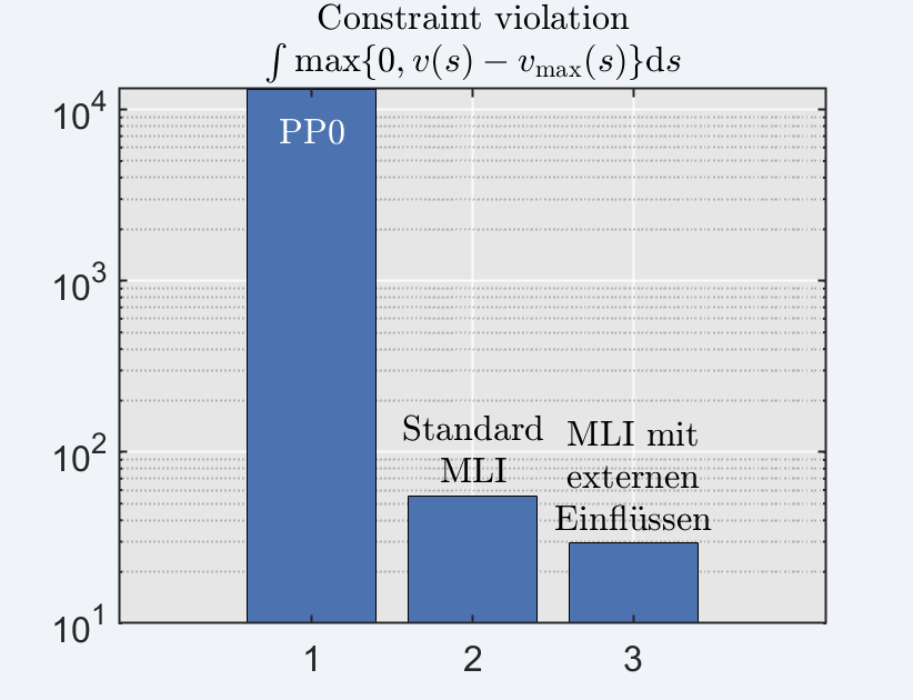
VIEL BESSERE EINHALTUNG DES TEMPOLIMITS!
11/14
Energieeffizientes Verfolgen von PP0
Energieeffizientes Befolgen
des Tempolimits
Ihno Schrot — Efficient Numerical Methods for NMPC with Applications in ACC — Disputationsvortrag — 03. Juli 2025
MEINE BEITRÄGE
4.
ANWENDUNG:
EACC
-
Realistisches Testproblem mit realen Kennfeldern und Fahrdaten
-
Erfolgreiche numerische Tests
STABILITÄT BEI INEXAKTEM NMPC
-
OCP semilinear parabolischer PDEs
-
Beweis asymptotischer Stabilität der System-Optimierer-Dynamik
FORM-ERHALTENDE
INTERPOLATION
-
Klassifikation im multivariaten Fall
-
Methode zur multivariaten, form-erhaltenden, glatten Interpolation
-
Berücksichtigung externer Einflüsse bei DMS, RTI und MLI
-
Angepasste Condensing-Strategien
EXTERNE EINFLÜSSE
-
Szenariobasiertes Online-Feedback
-
Online-Aufwand: Matrix-Vektor-Multiplikation oder Lösen eines QPs
SensEIS
FEEDBACK
12/14
Ihno Schrot — Efficient Numerical Methods for NMPC with Applications in ACC — Disputationsvortrag — 03. Juli 2025
STABILITÄT VON INEXAKTEM NMPC FÜR SEMILINEARE PARABOLISCHE PDEs
\newcommand{\ud}{\mathrm{d}}
\begin{aligned}
&\min_{x(\cdot),u(\cdot)} & \int_{t^j}^{t^j+T} &\Psi\left(x(t),u(t)\right) \ud t +
\Phi\left(x(t^j+T)\right)\\
&\quad\text{s.\,t. }& \dot{x}(t) &= f\left(x(t),u(t)\right),\quad t\in[t^j,t^j+T],\\
&& x(t^j) &= x^j,&&\\
&& 0 &\leq h\left(x(t),u(t)\right),\quad t\in[t^j,t^j+T],\\
&& 0 &= r^{\mathrm{e}} \left(x(t^j),x(t^j+T)\right),\\
&& 0 &\leq r^{\mathrm{i}} \left(x(t^j),x(t^j+T)\right).
\end{aligned}
ODE OPTIMALSTEUERUNGSPROBLEM
MOTIVATION: Stabilität Grundvoraussetzung für Sicherheit
ODE-FALL: Stabilität bewiesen, s. bspw. [Zanelli et. al, 2021]
- [Zanelli et. al., 2021] A. Zanelli, Q. Tran-Dinh, and M. Diehl. “A Lyapunov function for the combined system-optimizer dynamics in inexact model predictive control”. In: Automatica 134 (2021), p. 109901
-
[Tröltzsch, 2009] Optimale Steuerung partieller Differentialgleichungen: Theorie, Verfahren und Anwendungen. 2., überarb. Aufl. Studium. Wiesbaden: Vieweg + Teubner, 2009
Semilineare parabolische PDE
Semilineare parabolische PDE
Rand-steuerung
(aus [Tröltzsch, 2009])
\newcommand{\ud}{\mathrm{d}}
\begin{aligned}
&\min & &\int_{\Omega}\Phi\left(x,y\left(x,T\right)\right)\ud x + \iint_{Q}\phi\left(x,y\left(x,t\right)\right)\ud x\ud t\\
& &&+\iint_{\Sigma}\Psi\left(x,y\left(x,t\right),u\left(x,t\right)\right)\ud x\ud t\\
&\text{over}&&y\in C\left(\bar{Q}\right),\,u\in L^s\left(\Sigma\right),\\
&\text{s.\,t.}&&
\begin{aligned}
\dot{y}-\Delta y + f\left(x,y\right)&=0&&\text{in}~Q,\\
y(0) &= y^j &&\text{in}~\Omega,\\
\partial_\nu y + g\left(x,y\right)&=u&&\text{in}~\Sigma,\\
u_\mathrm{l}(x)\leq u\left(x,t\right)&\leq u_\mathrm{u}(x)&&\text{a.\,e.}~\Sigma.
\end{aligned}
\end{aligned}
PDE OPTIMALSTEUERUNGSPROBLEM
13/14
MEIN BEITRAG:
Inexakte NMPC Methoden auch bei PDEs stabil
Ihno Schrot — Efficient Numerical Methods for NMPC with Applications in ACC — Disputationsvortrag — 03. Juli 2025
STABILITÄT VON INEXAKTEM NMPC FÜR SEMILINEARE PARABOLISCHE PDEs
-
[Tröltzsch, 2009] Optimale Steuerung partieller Differentialgleichungen: Theorie, Verfahren und Anwendungen. 2., überarb. Aufl. Studium. Wiesbaden: Vieweg + Teubner, 2009
SYSTEM-OPTIMIERER-DYNAMIK
y^j = y\left(T;y^{j-1},u^{j-1}\right)
u^{j} = \xi\left(y^j,u^{j-1}\right)
System-
verhalten
System-
verhalten
Optimierer-
iteration(en)
u^{j-1}
y^{j-1}
Systemzustand
Steuerung
Optimierer-
iteration(en)
MEIN THEOREM
Der Gleichgewichtspunkt \( \left(y^\ast, u^\ast\right) = \left(0,0\right)\in L^p\left(\Omega\right)\times L^s\left(\Sigma\right) \) ist asymptotisch stabil für die System-Optimierer-Dynamik.
(aus [Tröltzsch, 2009])
\newcommand{\ud}{\mathrm{d}}
\begin{aligned}
&\min & &\int_{\Omega}\Phi\left(x,y\left(x,T\right)\right)\ud x + \iint_{Q}\phi\left(x,y\left(x,t\right)\right)\ud x\ud t\\
& &&+\iint_{\Sigma}\Psi\left(x,y\left(x,t\right),u\left(x,t\right)\right)\ud x\ud t\\
&\text{over}&&y\in C\left(\bar{Q}\right),\,u\in L^s\left(\Sigma\right),\\
&\text{s.\,t.}&&
\begin{aligned}
\dot{y}-\Delta y + f\left(x,y\right)&=0&&\text{in}~Q,\\
y(0) &= y^j &&\text{in}~\Omega,\\
\partial_\nu y + g\left(x,y\right)&=u&&\text{in}~\Sigma,\\
u_\mathrm{l}(x)\leq u\left(x,t\right)&\leq u_\mathrm{u}(x)&&\text{a.\,e.}~\Sigma.
\end{aligned}
\end{aligned}
PDE OPTIMALSTEUERUNGSPROBLEM
13/14
MEIN BEITRAG:
Inexakte NMPC Methoden auch bei PDEs stabil
Ihno Schrot — Efficient Numerical Methods for NMPC with Applications in ACC — Disputationsvortrag — 03. Juli 2025
STABILITÄT VON INEXAKTEM NMPC FÜR SEMILINEARE PARABOLISCHE PDEs
SYSTEM-OPTIMIERER-DYNAMIK
y^j = y\left(T;y^{j-1},u^{j-1}\right)
u^{j} = \xi\left(y^j,u^{j-1}\right)
System-
verhalten
System-
verhalten
Optimierer-
iteration(en)
u^{j-1}
y^{j-1}
Systemzustand
Steuerung
Optimierer-
iteration(en)
MEIN THEOREM
Der Gleichgewichtspunkt \( \left(y^\ast, u^\ast\right) = \left(0,0\right)\in L^p\left(\Omega\right)\times L^s\left(\Sigma\right) \) ist asymptotisch stabil für die System-Optimierer-Dynamik.
WICHTIGE ZWISCHENSCHRITTE IM BEWEIS
Schritt 1: Zustände bleiben im Level-Set \(\mathcal{Y}_{\bar{V}}\) einer Lyapunov-Fkt. und Steuerungen im Kontraktionsgebiet des Optimierers
\begin{align*}
&y^{0}\in\mathcal{Y}_{\bar{V}},&&u^{\mathrm{init}}\in\mathcal{B}_{\Sigma,s}\left(u^\ast\left(y^{0}\right),r_u\right)\\
\Rightarrow~ &y^{j+1}\in\mathcal{Y}_{\bar{V}},&&u^{j}\in\mathcal{B}_{\Sigma,s}\left(u^\ast\left(y^{j+1}\right),r_u\right)
\end{align*}
Schritt 2: Abschätzungen für Kontraktion des Steuerungs-fehlers \(E^j\) und der modifizierten Lyapunov-Fkt. \(V^j\), wobei
\begin{gather*}
E^j\coloneqq ||u^j-u^\ast\left(y^j\right)||_{L^s\left(\Sigma\right)},~V^j\coloneqq V\left(y^j\right)^{\frac{1}{q}}
\end{gather*}
Schritt 3: Asymptotische Stabilität des positiven, linearen Systems für die oberen Schranken \(E^j_\mathrm{u}\), \(V^j_\mathrm{u}\) gegeben durch
\begin{gather*}
\begin{pmatrix} V^{j+1}_{\mathrm{u}} \\ E^{j+1}_\mathrm{u}\end{pmatrix}=\begin{pmatrix}C_4 & C_3 \\ \kappa^k C_2 & \kappa^k C_1\end{pmatrix}\begin{pmatrix} V^{j}_{\mathrm{u}} \\ E^{j}_\mathrm{u}\end{pmatrix}~\text{mit}~\begin{pmatrix} V^{0}_{\mathrm{u}} \\ E^{0}_\mathrm{u}\end{pmatrix}=\begin{pmatrix} V^{0} \\ E^{0}\end{pmatrix}
\end{gather*}
13/14
MEIN BEITRAG:
Inexakte NMPC Methoden auch bei PDEs stabil
Ihno Schrot — Efficient Numerical Methods for NMPC with Applications in ACC — Disputationsvortrag — 03. Juli 2025
MEINE BEITRÄGE
ANWENDUNG:
EACC
-
Realistisches Testproblem mit realen Kennfeldern und Fahrdaten
-
Erfolgreiche numerische Tests
STABILITÄT BEI INEXAKTEM NMPC
-
OCP semilinear parabolischer PDEs
-
Beweis asymptotischer Stabilität der System-Optimierer-Dynamik
FORM-ERHALTENDE
INTERPOLATION
-
Klassifikation im multivariaten Fall
-
Methode zur multivariaten, form-erhaltenden, glatten Interpolation
-
Berücksichtigung externer Einflüsse bei DMS, RTI und MLI
-
Angepasste Condensing-Strategien
EXTERNE EINFLÜSSE
-
Szenariobasiertes Online-Feedback
-
Online-Aufwand: Matrix-Vektor-Multiplikation oder Lösen eines QPs
SensEIS
FEEDBACK
14/14
PhD_Defense
By Ihno Schrot


