Aim 3: Posterior Sampling and Uncertainty
September 12, 2023
Posterior Sampling Strategies Overview
\nabla_x \log~p_t(x_t | y) = \nabla_x \log~p_t(x_t) + \nabla_x \log~p_t(y | x_t)
\(\uparrow\)
SNIPS, DDRM: Analytically for linear forward models
[Jalal, 21]: Approximation for noiseless setting
\(\uparrow\)
Unconditional score network
\(\uparrow\)
Intractable in general
1. Ignore and project onto data manifold
[Chung, 21][Chung, 22][Song, 22]
2. Estimate it: DPS, \(\Pi\)DGM, ReSample
\(x_0\)
\(x_t\)
\(y\)
Intractability of \(p_t(y | x_t)\)
\(x_0\)
\(x_t\)
\(y\)
for the graphical model above
\[x_t \perp \!\!\! \perp y \mid x_0\]
p_t(y | x_t) = \int_{x_0} p(x_0 | x_t)p(y | x_0)\text{d}x_0
\(\uparrow\)
tractable
\(\uparrow\)
need to sample from entire diffusion model
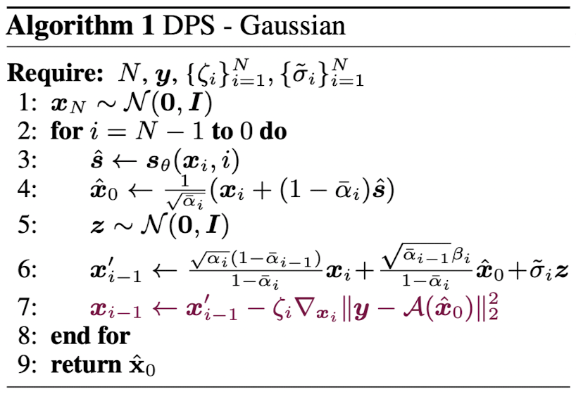
Diffusion Posterior Sampling (DPS) [Chung, 23]
p_t(y | x_t) = \mathbb{E}_{x \sim p(x_0 | x_t)}[p(y | x)]
estimate \(p_t(y | x_t)\) by pushing expectation in
p_t(y | x_t) \approx p(y | \hat{x}_0),~\hat{x}_0 \coloneqq \mathbb{E}_{x \sim p(x_0 | x_t)}[x]
can be written in closed-form via Tweedie's formula
Diffusion Posterior Sampling (DPS) [Chung, 23]
y = \mathcal{A}(x_0) + v,~v \sim \mathcal{N}(0, \sigma^2\mathbb{I})
\log p(y | x_t) \approx \log p(y | \hat{x}_0(x_t))\\
\implies \nabla_x \log p(y | x_t) \approx -\frac{1}{\sigma^2} \nabla_{x_t} \|y - \mathcal{A}(\hat{x}_0(x_t))\|^2_2
Diffusion Posterior Sampling (DPS) [Chung, 23]
y = \mathcal{A}(x_0) + v,~v \sim \mathcal{N}(0, \sigma^2\mathbb{I})
\log p(y | x_t) \approx \log p(y | \hat{x}_0(x_t))\\
\implies \nabla_x \log p(y | x_t) \approx -\frac{1}{\sigma^2} \nabla_{x_t} \|y - \mathcal{A}(\hat{x}_0(x_t))\|^2_2
\(\mathcal{A}\) can be nonlinear as long as it is differentiable
performance is very brittle to choice of \(\zeta_i\)
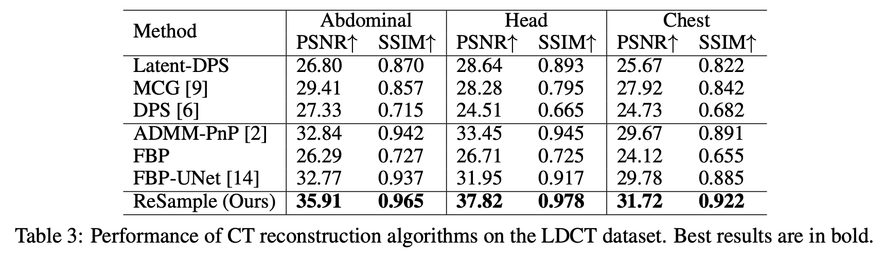
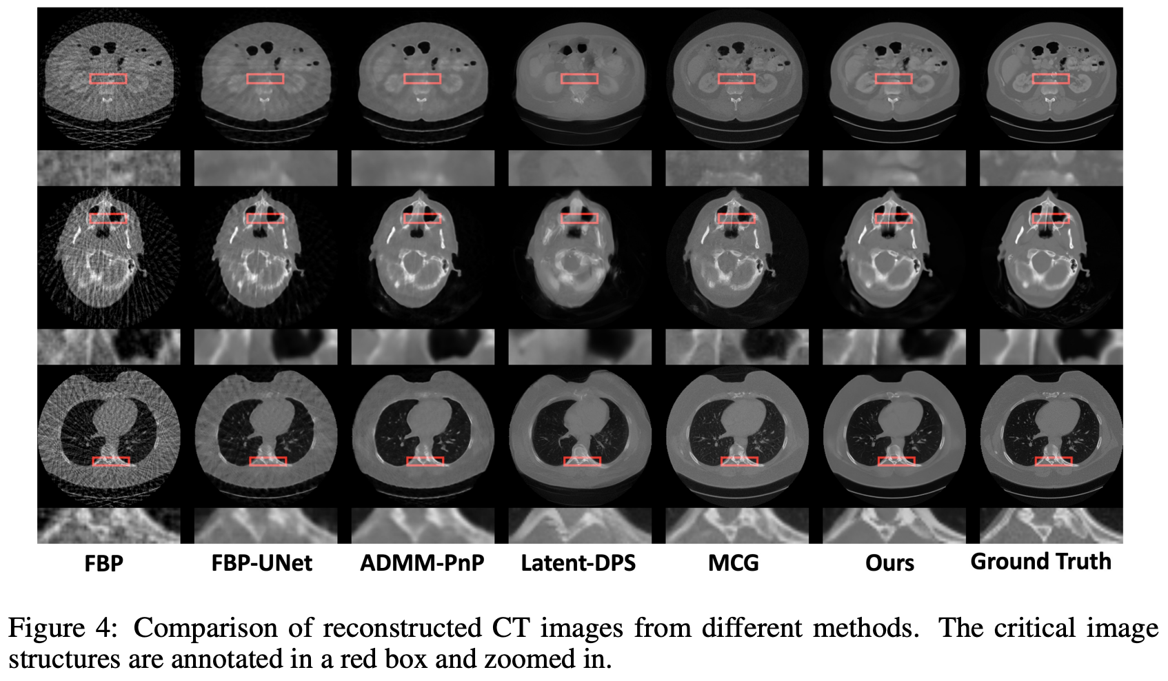
ReSample [Song, 23]
Latent-DPS
\[\mathcal{E}:~\mathbb{R}^d \to \mathbb{R}^k,~ \mathcal{D}:~\mathbb{R}^k \to \mathbb{R}^d\]
with
\[z = \mathcal{E}(x),~x = \mathcal{D}(z),~k \ll d\]
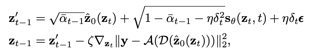
ReSample [Song, 23]
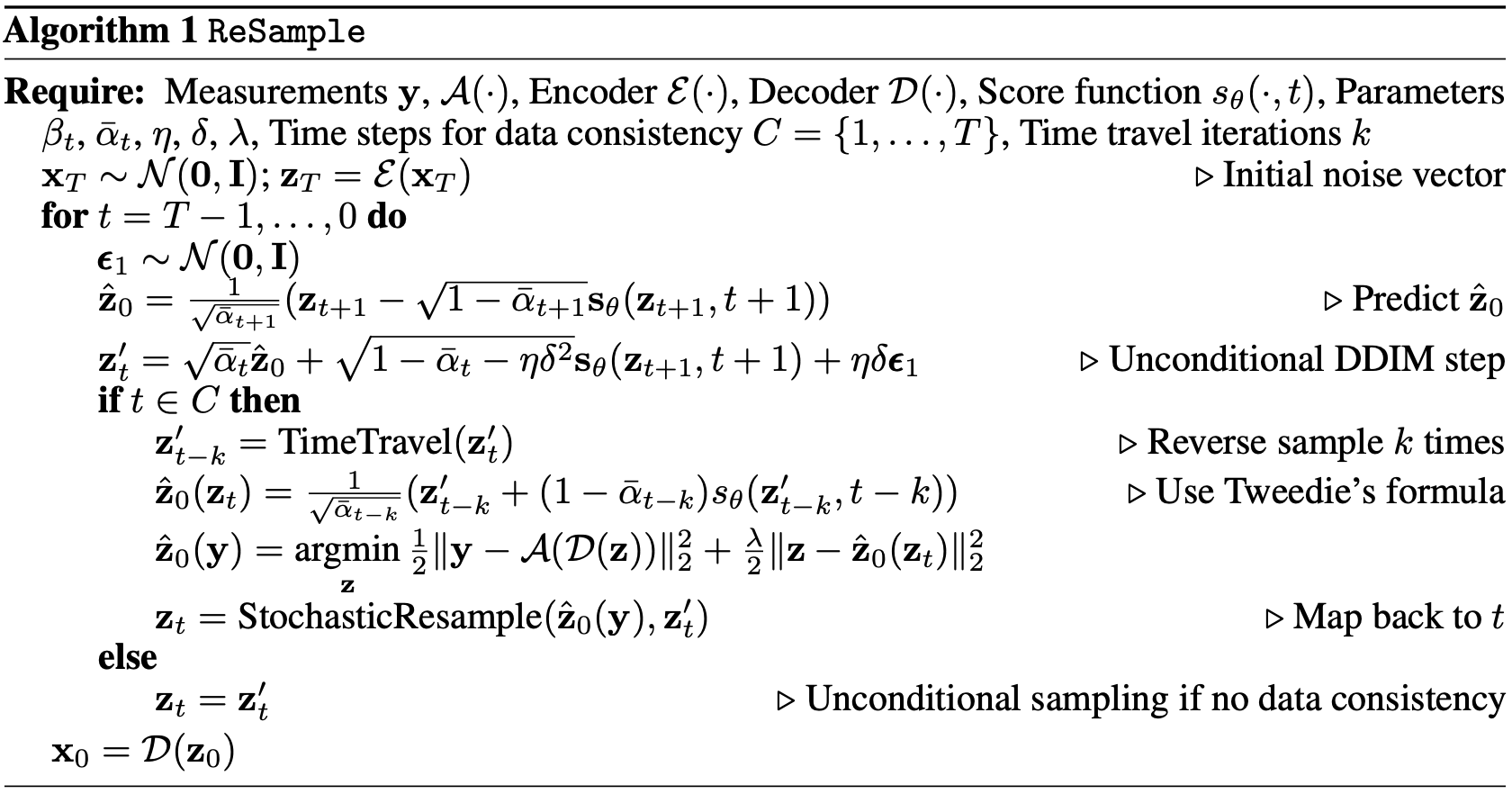
ReSample [Song, 23]
ReSample [Song, 23]
simulated sinograms with parallel-beam geometry with 25 projection angles over 180 degrees
\(\Pi\)GDM [Song, 23]
Recall
\[p_t(y | x_t) = \int_{x_0} p(x_0 | x_t)p(y | x_0)\text{d}x_0\]
and assume
\[p(x_0 | x_t) \approx \mathcal{N}(\hat{x}_0, r^2_t\mathbb{I})\]
Suppose
\[y = Hx_0 + v,~v \sim \mathcal{N}(0, \sigma^2_y\mathbb{I})\]
then
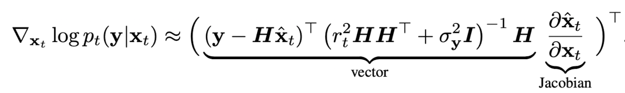
\(\Pi\)GDM [Song, 23]
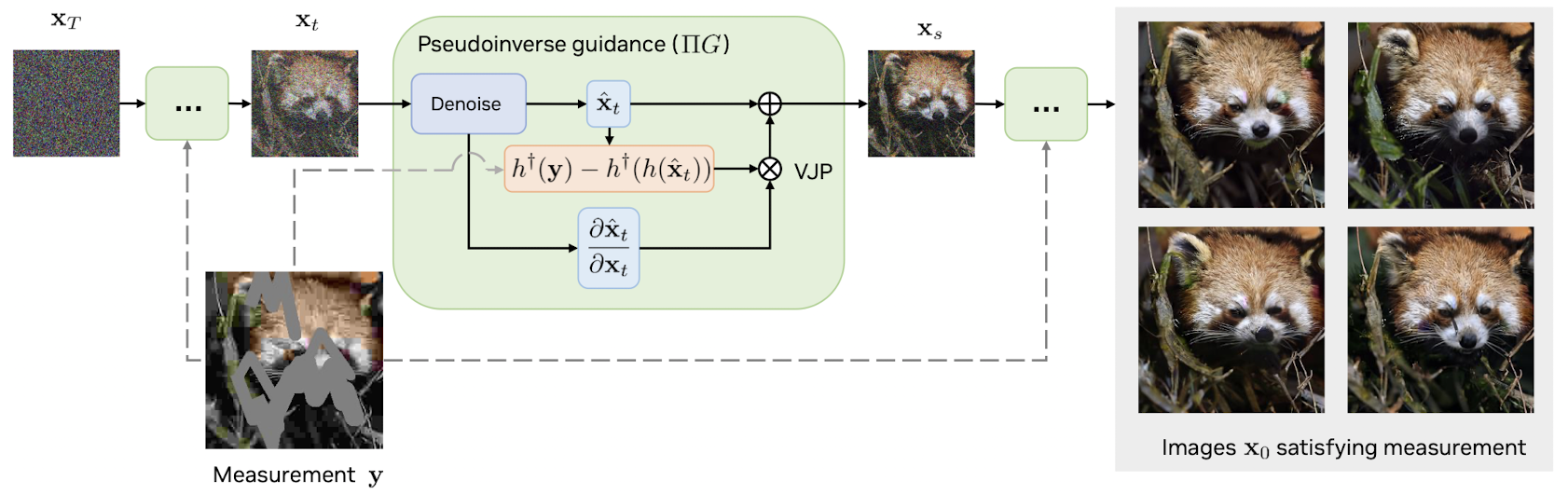
For a general noiseless forward function \(h\) with
\[h(h^\dagger(h(x))) = x\]
\(h\) need not be differentiable
does not require tuning of stepsize
Fourier Diffusion Models [Tivnan, 23]
\(x_0\)
\(x_t\)
\(y\)
forward process converges to the measurement model distribution
reverse sampling is unconditional sampling but the model works for one forward process only
LoDoPaB-CT Dataset [Leuschner, 21] [link]
Based on the TCIA LIDC-IDRI Dataset [link]
\[y = - \ln\left(\frac{n_{x_0}}{n_0}\right),\quad~n_{x_0} \sim \text{Pois}(n_0e^{-Ax_0})\]
\(x_0\): 40keV ground-truth image (in HU)
\(A\): forward operator
\(n_0\): expected number of photons with no attenuation
Note that in the noiseless setting
\[y = Ax_0\]
as expected
LoDoPaB-CT Dataset [Leuschner, 21] [link]
\(A\) implemented with the ODL package [link]
\(xy\) spatial resolution = 0.5 mm, image size = 512 pixels \(\implies\) domain = 25.6 cm.
1000 angles and 512 detectors
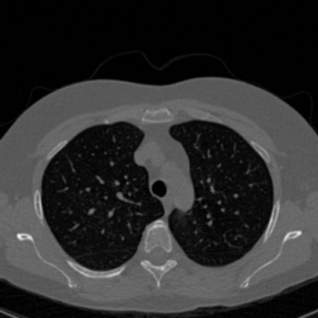
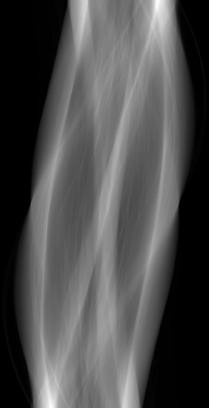

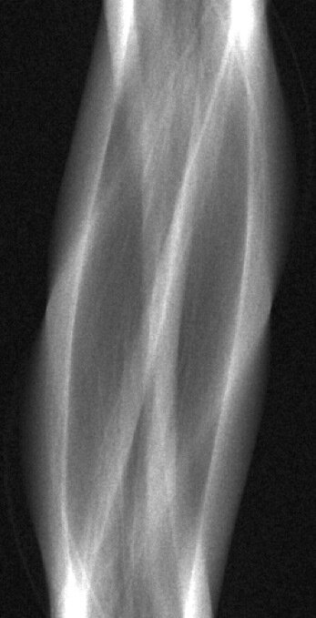
40 keV ground-truth
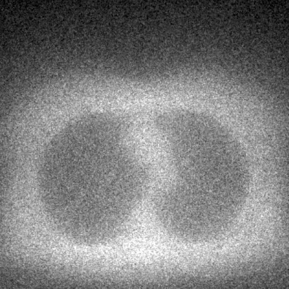
sinogram
FBP reconstruction
LoDoPaB-CT Dataset [Leuschner, 21] [link]
Simulated observations and FBP reconstructions
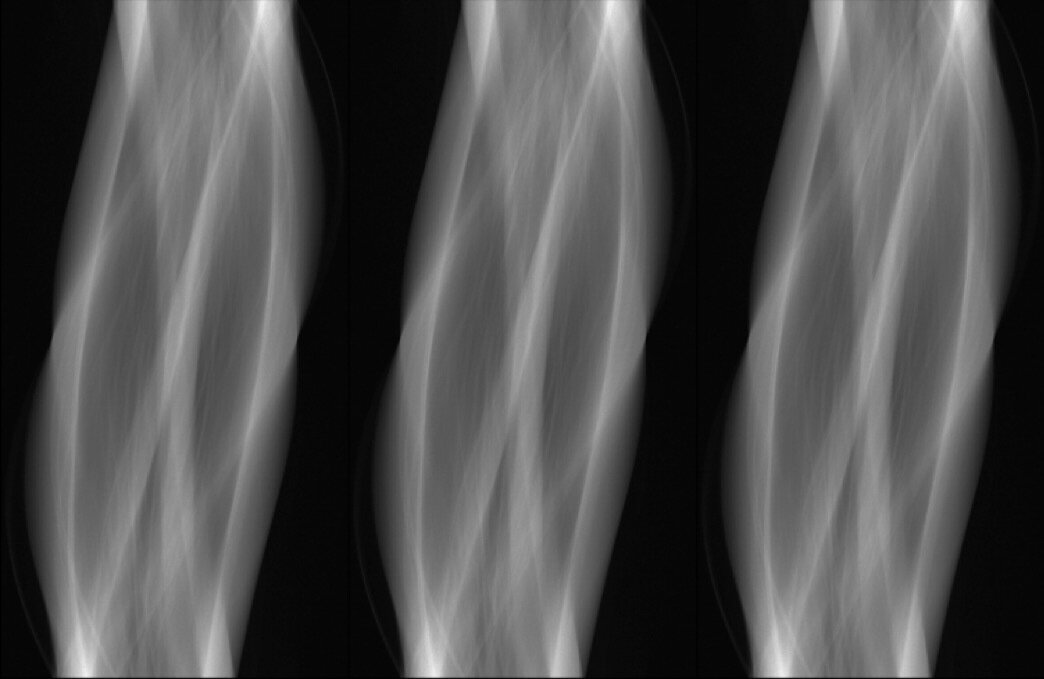
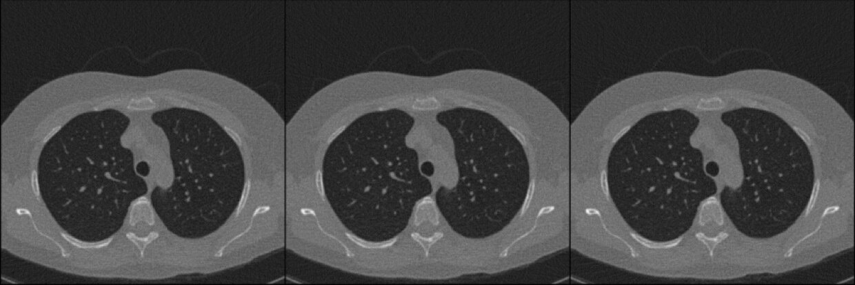
ground-truth
simulated observations & reconstructions
-
-
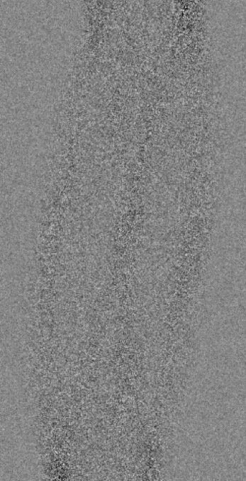

std
mean
=
=
The Conditional Score is Invariant
to Change of Variable
Recall
\[y = - \ln\left(\frac{n_{x_0}}{n_0}\right) = f(n_{x_0}) \neq Ax_0 + v\]
by change of variable rule
\[g(x) = f^{-1}(x)\]
and
\[p(y \mid x_0) = p(n_{x_0} = g(y)) \cdot (-g'(y))\]
\[\implies \nabla_{x_0} \log p(y \mid x_0) = \nabla_{x_0} \log p(n_{x_0} = g(y))\]
The Conditional Score is Invariant
to Change of Variable
Recall
\[y = - \ln\left(\frac{n_{x_0}}{n_0}\right) = f(n_{x_0}) \neq Ax_0 + v\]
let
\[g(x) = f^{-1}(x)\]
and by change of variable rule
\[p(y \mid x_0) = p(n_{x_0} = g(y)) \cdot (-g'(y))\]
\[\implies \nabla_{x_0} \log p(y \mid x_0) = \nabla_{x_0} \log p(n_{x_0} = g(y))\]
\[\downarrow\]
Can Use DPS Approximation
\[\nabla_{x_t} \log p(y \mid x_t) \approx \nabla_{x_t} \log p(y \mid \hat{x}_0(x_t)) = \nabla_{x_t} \log p(n_{\hat{x}_0(x_t)} = g(y))\]
Next Steps
Implement CT Measurement model on:
- lung: LoDoPaB-CT
- abdomen: AbdomenCT-1K
- brain: RSNA ICH Challenge
Train diffusion models for each dataset:
- Both VP & VE SDE (LoDoPaB-CT/VP in progress)
Implement conditional sampling strategies
- Modified DPS
- How to modify \(\Pi\)GDM without normal approx?
[09/12/23] Aim 3: Posterior Sampling and Uncertainty
By Jacopo Teneggi


