Tensor Types & Categories
James B. Wilson, Colorado State University


Follow the slides at your own pace.
Open your smartphone camera and point at this QR Code. Or type in the url directly
https://slides.com/jameswilson-3/tensor-types-cats/#/

Major credit is owed to...

Uriya First
U. Haifa
Joshua Maglione,
Bielefeld
Peter Brooksbank
Bucknell
- The National Science Foundation Grant DMS-1620454
- The Simons Foundation support for Magma CAS
- National Secturity Agency Grants Mathematical Sciences Program
- U. Colorado Dept. Computer Science
- Colorado State U. Dept. Mathematics

Why care about categories?
\mathrm{Isom}(F_i)=\{ X:\mathbb{M}_d(K) \mid XF_iX^{\dagger}=F_i\}\\
\bigcap_{i=1}^n \mathrm{Isom}(F_i).
Problem: how to intersect large classical groups.
Quadratic equations in d^2 variables.
Genercially quadratic equations are as hard as all polynomial equations.
Obvious solution is Groebner basis which is impossibly hard even for d=4.
\mathrm{Isom}(F_i)=\{ X:\mathbb{M}_d(K) \mid XF_iX^{\dagger}=F_i\}\\
\bigcap_{i=1}^n \mathrm{Isom}(F_i).

Isometry is equivalence in this cateogry (columns are objects.)
But what if we look at a different category?
The Adjoint category:
(a_2)\phi_2*b_1 = a_2\circ \phi_1(b_1)
- The adjoint category is abelian.
- Endomorphisms form a ring (computable).
- Isomorphisms are units of a ring (computable).
Isomorphism in Isometry category is THE SAME as isomorphism in adjoint category
Just flip the arrow -- legal because with isomorphism arrows are invertible.
Categories matter because they let us change the question, and see something different to try.
They also are critically helpful in making useful programs.
Objectives
- All the right types
- Noether's Isomorphisms
- Functors
- A representation theory
x:A \equiv \textnormal{Claim } x\in A \textnormal{ with proof of the claim.}\qquad\qquad\qquad\\
\qquad \equiv \textnormal{Data created/used by type rules A (e.g. 32-bit float)}
(a:A) \to (b:B) \to (f(a,b):C)\\
\qquad\equiv f:A\to (B\to C)\\
\qquad\equiv f:A\to B\to C\\
\qquad \equiv f:A\times B\to C
( P \Rightarrow Q ) \textnormal{ often same as functions } (x:P)\to (y:Q)
Notation Choices
Below we explain in more detail.
[a] = \{0,\ldots,a\}
Notation Motives
Mathematics Computation
Vect[K,a] = [1..a] -> K
$ v:Vect[Float,4] = [3.14,2.7,-4,9]
$ v(2) = 2.7

*:Vect[K,a] -> Vect[K,a] -> K
u * v = ( (i:[1..a]) -> u(i)*v(i) ).fold(_+_)
K^a = \{v:\{1,\ldots,a\}\to K\}
\mathbb{M}_{a\times b}(K) = \{ M:\{1,\ldots,a\}\times \{1,\ldots,b\}\to K\}
\cdot:K^a\times K^a\to K\qquad\\
u\cdot v = u_1v_1+\cdots+u_a v_a
\cdot:\mathbb{M}_{a\times b}(K) \times K^b\to K^a\\
M\cdot v =
\begin{bmatrix}
M_{1}\cdot v\\
\vdots\\
M_{a}\cdot v
\end{bmatrix}
Matrix[K,a,b] = [1..b] -> Vect[K,a]
$ M:Matrix[Float,2,3] = [[1,2,3],[4,5,6]]
$ M(2)(1) = 4


*:Matrix[K,a,b] -> Vect[K,b] -> Vect[K,a]
M * v = (i:[1..a]) -> M(i) * v
Difference? Math has sets, computation has types.
But types are math invention (B. Russell); lets use types too.
A type for Tensors
Definition. A tensor space is a linear map from a vector space into a space of multilinear maps.
\langle \cdot | : T\to V_0\oslash\cdots\oslash V_{\ell}\\
\qquad\qquad\qquad\qquad=\{f:V_{\ell}\to (\cdots\to V_0)\}
Tensors are elements of a tensor space.
The frame is
The axes are the
The valence is the the size of the frame.
V_*:(a:[\ell])\to (V_a:\mathsf{VectSpace})
V_a
Naïve Tensors: Lists of lists
You type this:
t = [[ 3, 1, 0 ],[ 0, 3, 1 ],[ 0, 0, 3 ]]
You're thinking of:
\begin{bmatrix}
3 & 1 & 0 \\
0 & 3 & 1 \\
0 & 0 & 3
\end{bmatrix}
But your program plans for:
\begin{bmatrix}
~[ 3, 1, 0, 9, 8 ], \\
~[ ], \\
~[ x, car, @ ]
\end{bmatrix}
Effect: your program stores your data all-over in memory heap and slows down to double-check your instructions.
Details.
Memory Layout Problems
In a garbage collected systems (Java/Python/GAP/Magma
/Sage...) objects are stored on a heap - e.g. a balanced (red/black) tree.
Separate data like rows in a list of lists are therefore placed into the heap in the place that balances the tree.
While lookups are logarithmic, because your data is spread out but only ever used together, you add slow down.
Memory Access Problems
The more structured your data structure the more complex the lookup.
In a list of lists what you actually have is a pointer/reference to on address in memory for each row.
Within a list you can just add 1, 2, etc. to step the counter through the row.
However, if you intend to step through columns you jump around memory -- may force machine to load data in and out of cache.
Index bounds
Languages like Java/Python/GAP/Magma etc. need to confirm that you never access an entry outside the list.
So A[i][j][k] is in principal checking that i, j, and k are each in the right bounds.
As a list of lists, many systems cannot confirm that j is in range until it has the correct row (recall the computer prepares for uneven rows!) This is true even for most compiled languages.
Result: bounds are checked at runtime, even if you know they are not needed.

Abacus Tensors
Solution: separate the data from the grid.
Tensors are any element of a tensor space so as long as they can be interpreted as multilinear they are indeed tensors. No grids needed.
Abacus Tensor Contraction
\langle t | v_2,v_1\rangle = \sum_{i=0}^{d_2-1}\sum_{j=0}^{d_1-1} t[i\cdot d_1+j]\cdot v_2[i]v_1[j]
Math is this:
See how we often access entire regions contiguously or by arithmetic progression.
Bad idea: perform arithmetic for each index lookup!
Quickly that work costs more than the actual tensor contraction.
Indices of abacus tensors
t[i_{\ell} d_{\ell-1}\cdots d_0+\cdots + i_1\cdot d_0+i_0]
Math is this:
Step through indices with an "abacus machine", e.g. Minsky Annals Math, 1960.
These are Turing complete computational models that are based on numbers -- not symbols -- so arithmetic is the program.
Never heard of one? Oh, its simply the registers AX, BX, ... with on x86 compatible microprocessor!
Safe Index Lookup
Problem: Checking bounds required only if computer cannot prove (before run-time) that we are in range.
Solution: don't give an index, give a proof!
t:Tensor 10 20 = ...
t[i+j=10][1<=k<=20]

t:Tensor a b = ...
t[i+j=a][1<=k<=b]
"=" and "<=" are data, proofs are data!
Even data based on variables allowed -- says when values are given they will conform to the stated structure.
The computer (compiler) can then safely remove all checks.
But requires a dependent type system.
3:\mathbb{N} \equiv \textnormal{Claim }3\in \mathbb{N}. \textnormal{ Proof: } 3=SSS0.
Taste of Types
\mathbb{N} = 0 | S(n:\mathbb{N})
x\in \{n\in \mathbb{N}\mid (\exists k)(n=k+k)\}\qquad\qquad\\
\qquad \Rightarrow x+1\in \{n\in \mathbb{N}\mid (\exists k)(n=1+k+k)\}
\mathsf{Even} <: \mathbb{N} = 0 ~|~ n+n\quad\\
\mathsf{Odd} <: \mathbb{N} = S(n:\mathsf{Even})\\
(n:\mathsf{Even}) \longrightarrow (S(n):\mathsf{Odd})
Terms of types store object plus how it got made
Implications become functions
hypothesis (domain) to conclusion (codomain)
(Union, Or) becomes "+" of types
(Intersection,And) becomes dependent type
x\in A\cup B \Leftrightarrow x:(A+B)\\
x\in \bigcup_{i\in I} A_i \Leftrightarrow x:\sum_{i:I} A_i\\
x\in A\cap B \equiv x:A\times B\\
x\in \bigcap_{i\in I} A_i \Leftrightarrow x: \prod_{i:I} A_i \equiv x:(i:I)\to (x_i:A_i)
Types are honest about "="
K[x_1,\ldots,x_n]/(f_1,\ldots,f_m) = K[x_1,\ldots,x_n]/(g_1,\ldots,g_k)
Sets are the same if they have the same elements.
Are these sets the same?
We cannot always answer this, both because of practical limits of computation, but also some problems like these are undecidable (say over the integers).
In types the above need not be a set.
Sets are types where a=b only by reducing b to a explicitly.
Do types slow down my code?
Quite the opposite: despite adding potentially more lines to your code, think of those as instructions to the compiler on how to remove any unnecessary steps at runtime. (The axioms of unique choice implies you can remove all the line-by-line proofs in process known as "erasure".)
Bonus: programming this way means when it works, you have a rigorous math proof that your code is what you claim.
Other Primitives
Stacking/Slicing an Abacus Tensor
To stack: add a wire and move right number of beads. Do vice-versa to slice.

Shuffle an Abacus Tensor
Swap the wires.
Tensor Product
Take the disjoint union of axes abaci!

Avoids writing to memory what in the end is just a bunch of repeated information. Less information to move/store, and easy to recompute.
Other types of tensors
- Formulas: e.g. associator or commutator of an algebra.
- Polarization of polynomials.
- Commutation in a group.
- Sparse linear combinations of tensors
Main Point
Tensor as elements of tensor spaces can therefore be represented by any data structure appropriate to your task. Use that to your advantage.
Tensor Categories
(V_0:\mathsf{Abel})\to (V_1:\mathsf{Abel})\longrightarrow (V_0\oslash V_1:\mathsf{Abel})
Versors
@: V_0\oslash V_1 \times V_1 \to V_0 \\
@(f+f',v_1)=@(f,v_1)+@(f',v_1)\\
@(f,v_1+v'_1) = @(f,v_1)+@(f,v'_1)\\
\hom(V_2,\hom(V_1,V_0))\to \hom(V_2,V_0\oslash V_1)
1. An abliean group constructor (perhaps just an additive category?)
2. Together we a distributive "evaluation" function
3. Universal Mapping Property
V_0\oslash V_1 \times V_1 \to V_0\qquad (f,v_1)\mapsto f(v_1)
Versors: an introduction
V_0\oslash V_1 = \{ f:V_1\to V_0\mid f(v_1+v'_1)=f(v_1)+f(v'_1)\}
Why the notation? Nice consequences to come, like...
(V_0\oslash V_1)\otimes_{\mathrm{End}(V_1)} V_1 \cong V_0\\
Context: finite-dimensional vector spaces
Actually, versors can be defined categorically
V_0\oslash V_1\oslash V_2 = (V_0\oslash V_1)\oslash V_2
Bilinear maps (bimaps)
f:V_0\oslash V_1\oslash V_2 \equiv f:V_2\to (V_1\to V_0)
(v_2:V_2) \to (f(v_2):V_0\oslash V_1)
(v_2:V_2) \to (v_1:V_1) \to (f(v_2)(v_1):V_0)\\
f:V_2\times V_1 \rightarrowtail V_0\\
(\rightarrowtail\textnormal{ to indicate multi-linear})
Rewrite how we evaluate ("uncurry"):
Practice
M:\mathbb{M}_{2\times 3}(\mathbb{R})
\langle M| : \mathbb{R}^2\oslash \mathbb{R}^3 \equiv \langle M|:\mathbb{R}^3\to \mathbb{R}^2\\
(v:\mathbb{R}^3)\to (Mv: \mathbb{R}^2)\\
\langle M| v\rangle=Mv
\langle M|:\mathbb{R}^3\oslash \mathbb{R}^2 \equiv \langle M|:\mathbb{R}^2\to \mathbb{R}^3\\
(u:\mathbb{R}^2)\to (uM :\mathbb{R}^3)\\
\langle M|u\rangle=uM
\langle M| : \mathbb{R}\oslash \mathbb{R}^2\oslash\mathbb{R}^3 \equiv \langle M|:\mathbb{R}^3\to (\mathbb{R}^2\to \mathbb{R})\\
\qquad \equiv \langle M|:\mathbb{R}^3\times \mathbb{R}^2\to \mathbb{R}
(v_2:\mathbb{R}^3)\to (v_1:\mathbb{R}^2) \to (v_2Mv_1 : \mathbb{R})\\
\langle M|v_2\rangle |v_1\rangle=\langle M|v_2\rangle |v_1\rangle=v_2Mv_1
Practice with Notation
V_0\oslash \cdots\oslash V_{\ell}\qquad\qquad\qquad\\
\qquad = \{ f:V_{\ell}\to (\cdots\to V_0)\}\qquad\\
\qquad = \{ f:V_{\ell}\times \cdots\times V_1 \rightarrowtail V_0\}
Multilinear maps (multimaps)
\langle f| v_{\ell}\rangle \cdots | v_1\rangle = \langle f | v_{\ell},\ldots,v_1\rangle
Evaluation
Thesis:
Every concept in nonassociative algebra has a tensor analog.


Homotopisms
Recognizing the complexity of nonassociatie algebra, A. A. Albert introduced "isotope" as coarser equivalence:
f(a*b)=f(a)\circ f(b)
h(a*b)=f(a)\circ g(b)
Algebra isomorphism:
Category theory made all things "-isms" so now "isotopism", and more generally "homotopism".
Homotopisms of tensors
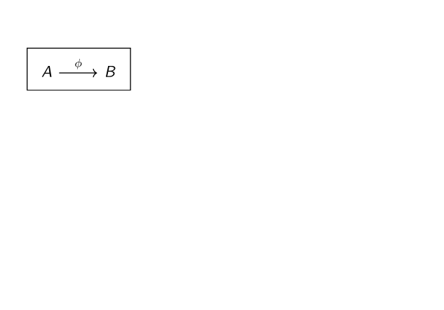
\phi:t\to s \equiv (\phi:\prod_{a:[\ell]} V_a\to U_a) \longrightarrow
\phi_0\langle t|v_{\ell},\ldots,v_1\rangle = \langle s|\phi_{\ell}v_{\ell},\ldots,\phi_1 v_1\rangle
In want of term for tensors we use Albert's.
(\phi:t\to s) \longrightarrow (\tau:s\to r) \longrightarrow (\phi\tau:t\to r)\\
(\phi\tau)_a=\phi_a\tau_a
Compose pointwise
(t:T)\to (\langle t|:V_0\oslash\cdots\oslash V_{\ell})\\
(s:S)\to (\langle s|:U_0\oslash\cdots\oslash U_{\ell})
Homotopisms include
- Algebra homomorphisms.
- Linear maps
- Isometries

Linear
Isometry
Yet not everything

Degeneracy
A_1^{\bot} =\{a_2:A_2\mid a_2*A_1=0\}\\
A_2^{\bot} =\{a_1:A_1\mid A_2*a_1=0\}\\
Most theorems fail/harder if we include tensors with degeneracy "all zero rows/columns".
Easy to remove.
But, that removal is not by a homotopism!
Adjoints
(\langle \phi_2(a_2),\phi_1(a_1)\rangle =\langle a_2,a_1\rangle)\to
(\langle \phi_2^{-1}(a_2), a_1\rangle = \langle a_2,\phi_1 a_1\rangle)
Isometries are immensely facilitated by considering adjoints instead.
But, adjoints are not homotopisms!
Further Categories
For tensors of valence n there are 2^n "self-evident" categories.
- Are we missing any?
- When are these equivalent?
- How to compute within them?
- Is this actually a single larger 2 or n-category?
- What kind of categories? Abelian when? Products? Projectives? Simples? Representation theory?
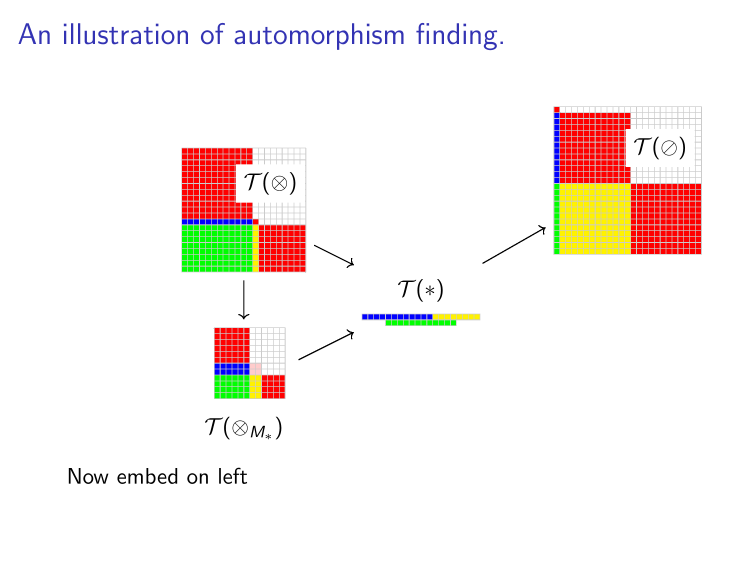
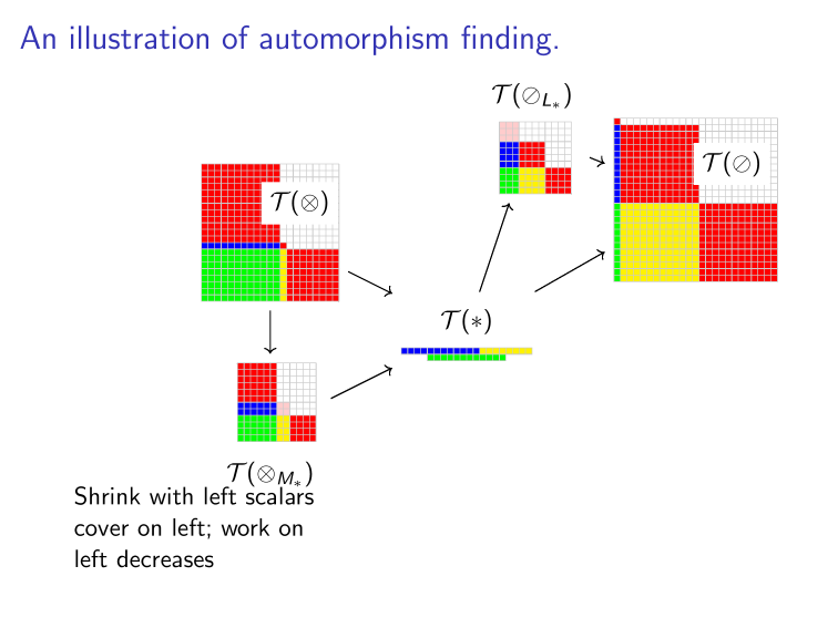
Classifying the Categories
Idea: endomorphisms in a category are monoids.
- Use our polynomial traits to classify all transverse operators that support monoids.
- Then check if any of those traits support categories.
(\rho:K[x_0,\ldots,x_{\ell}]\to \mathrm{End}(V_0\oslash\cdots\oslash V_{\ell}))
(\omega:\prod_a \mathrm{End}(V_a))\to
Claim
Kernel is the annihilator of the operator.
Theorem. A Groebner basis for this annihilator can be computed in polynomial time.
Annihilators General
\mathrm{ann}_{\omega}(t) = \{ a(X):K[X]\mid \langle t|a(X) =0 \}
a(X)=\sum_{e:[\ell]\to \mathbb{N}} \alpha_e X^e\longrightarrow \\
\qquad 0=\sum_{e} \alpha_e \omega_0^{e_0} \langle t | \omega_{\ell}^{e_{\ell}}v_{\ell},\ldots,\omega_1^{e_1} v_1\rangle

T(P,\Delta) = \{ t:T\mid \langle t| P(\Delta)|v\rangle =0\}
Sets of the Correspondence
Akin to eigen spaces:
I(S,\Delta) = \{ p:K[X]\mid \langle S| p(\Delta)|v\rangle =0\}
Akin to characteristic/minimal polynomial:
Z(S,P) = \{ \omega:\prod_a \mathrm{End}(V_a)\mid \langle S| P(\omega)|v\rangle =0\}
Akin to weights:

The Correspondence Theorem (First-Maglione-W.)
This is a ternary Galois connection.
Summary of Trait Theorems (First-Maglione-W.)
- Linear traits correspond to derivations.
- Monomial traits correspond to singularities
- Binomial traits are only way to support groups.
For trinomial ideals, all geometries can arise so classification beyond this point is essentially impossible.
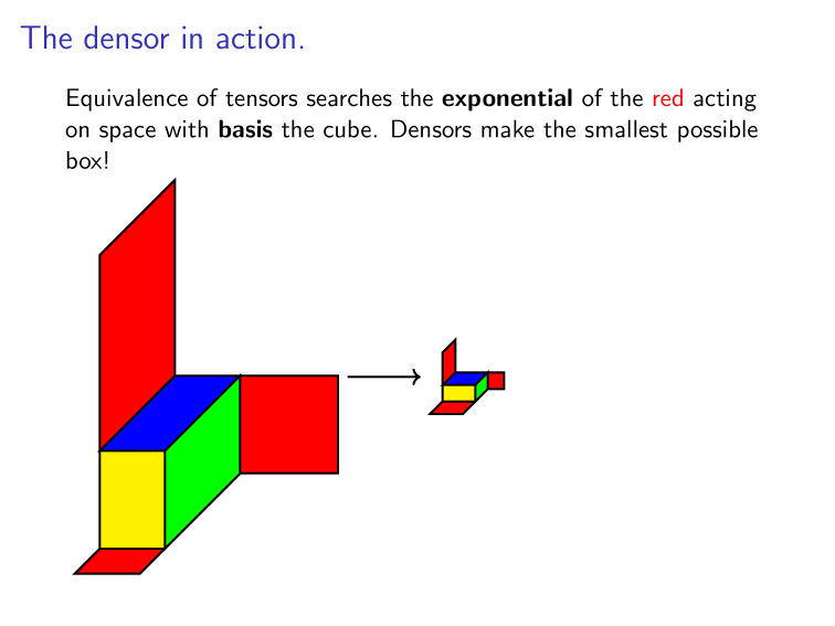
Derivations & Densors
Treating 0 as contra-variant the natural hyperplane is:
D(x_0,\ldots,x_{\ell}) = -x_0 + x_1+\cdots + x_{\ell}
That is, the generic linear trait is simply to say that operators are derivations!
\langle t | D(\delta) |v\rangle=0 \equiv\\
\delta_0 \langle t|v\rangle = \langle t|\delta_{\ell} v_{\ell},\cdots ,v_1\rangle+\cdots+\langle t|v_{\ell},\ldots,\delta_1 v_1\rangle
However, the schemes Z(S,P) are not the same as Z(P), so generic here is not the same as generic there...work required.
Derivations are Universal Linear Operators
Theorem (FMW). If
2.~ P=(\sum_{a} \alpha_{1a} x_a, \cdots, \sum_a \alpha_{ma} x_a)
Then
3.~(\forall a:[\ell])(\exists i:[m])(\alpha_{ia}\neq 0)
1. |K|>\ell
(\exists \omega:\prod_{a=0}^{\ell} K^{\times}) ( Z(S,P)^{\omega} <: \mathrm{Der}(S) )
(If 1. fails extend the field; if 2. is affine, shift; if 3 fails, then result holds over support of P.)
Tensor products are naturally over Lie algebras
Theorem (FMW). If
(\omega,\omega':Z(S,P)) \to\hspace{5cm}\\
\qquad(\omega_a\bullet \omega'_a = \alpha_{a}\omega_a\omega'_a+\beta_a \omega'_a\omega_a : Z(S,P))
Then in all but at most 2 values of a
\langle (\alpha_a,\beta_a)\rangle = \langle (1,-1)\rangle \textnormal{ i.e. a Lie bracket}
In particular, to be an associative algebra we are limited to at most 2 coordinates. Whitney's definition is a fluke.


Binomials & Groups
Theorem (FMW). If for every S and P
(\omega,\omega'\in Z(S,P))\to (a:[\ell])\to
((\omega_a\omega'_a)^{\pm 1}=:Z(S,P))
P=(X^{e_1}-X^{f_1},\ldots, X^{e_m}-X^{f_m})
(i,j:[1..m])\to (a:[\ell]) \to (e_i(a)+f_j(a)\leq 1)
then
If
then the converse holds.
(We speculate this is if, and only if.)
Binomial Tensor Categories.
X^e-X^f, e(a)+f(a)\leq 1.
Let operators act covariantly on support of e and contravariantly on support of f.
x_2 x_1-x_0
\phi_2(a_2)\circ\phi_1(a_1) = \phi_0 (a_2*a_1)\\
\langle s|\phi_2(a_2),\phi_1(a_1)\rangle = \phi_0\langle t|a_2,a_1\rangle\\

x_2 x_0-x_1
\phi_0(\phi_2(a_2)\circ a_1) = a_2*\phi_1(a_1)\\
\phi_0\langle s|\phi_2(a_2),a_1\rangle = \langle t|a_2,\phi_1(a_1)\rangle\\


BUT this is rather forced and adds in way more operators than those needed.
Is there a better idea to just glue the natural categories together without introduction morphisms we don't want?
Shuffle the Frames
\langle t^{(1,2)}| u_1,u_2\rangle = \langle t|u_2,u_1\rangle.

These are basis independent (in fact functors),
E.g.:
Rule: If shuffling through index 0, collect a dual.
\langle t^{(0,1)} |: V_2\times (K\oslash V_0) \rightarrowtail (K\oslash V_1)
\langle t^{(0,1)} | v_2, \nu_0\rangle|v_1\rangle = \nu_0\langle t|v_2,v_1\rangle.
And so duals applied in 0 and 1


Tensor Types & Categories
By James Wilson
Tensor Types & Categories
Primitive types and categories for tensors. CC-BY-2019 James B. Wilson


