Foundations of entropy in complex systems
ISING LECTURES-2026
28th Annual Workshop on Critical Phenomena and Complex Systems

Jan Korbel

Slides available at: slides.com/jankorbel
Personal web: jankorbel.eu

Warning!

CSH Vienna

Vienna, city of famous people
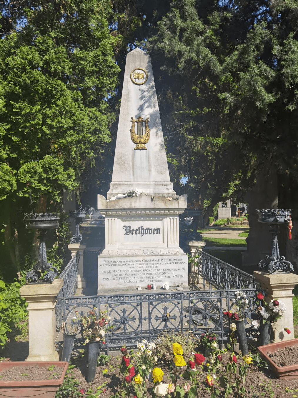
Beethoven
Udo Jürgens

\( S = k \cdot \log W\)
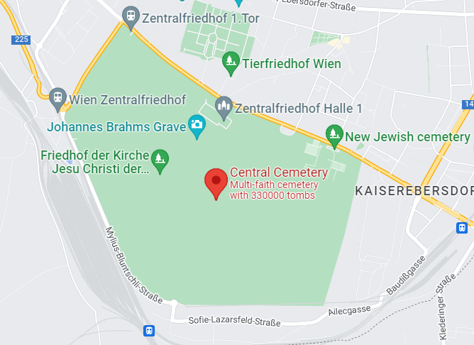
Where physicists go
This talk will show you how important is Boltzmann's formula for statistical physics of complex systems
From many to a few
- Most physical disciplines study the detailed prediction of physical systems, including their precise evolution in time
- They typically focus on systems composed of a few variables
- In physics, they are called degrees of freedom - DOF
- Examples of degrees of freedom:
- particle position \(x\)
- particle velocity \(v\)
- molecule angular momentum \(L\)
- For each degree of freedom, we have one (typically differential) equation that is interconnected with the other degrees of freedom
What if we have 1 mol (\(\approx 10^{23})\) particles?
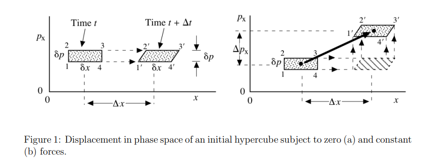
Liouville theorem
Let's have canonical coordinates \(\mathbf{q}(t)\), \(\mathbf{p}(t)\) evolving by Hamiltonian dynamics
$$\dot{\mathbf{q}} = \frac{\partial H}{\partial \mathbf{p}}\qquad \dot{\mathbf{p}} = - \frac{\partial H}{\partial \mathbf{q}}$$
Let \(\rho(p,q,t)\) be a probability distribution in the phase space. Then, \(\frac{\mathrm{d} \rho}{\mathrm{d} t} = 0.\)
Consequence: \( \frac{\mathrm{d} S(\rho)}{\mathrm{d} t}= - \frac{\mathrm{d}}{\mathrm{d} t} \left(\int \rho(t) \ln \rho(t)\right) = 0.\)
Useful results from statistics
1. Law of large numbers (LLN)
\( \sum_{i=1}^n X_i \rightarrow n \bar{X} \quad \mathrm{for} \ N \gg 1\)
2. Central limit theorem (CLT)
\( (\frac{1}{n} \sum_{i=1}^n X_i - \bar{X}) \rightarrow \frac{1}{\sqrt{n}} \mathcal{N}(0,\sigma^2)\)
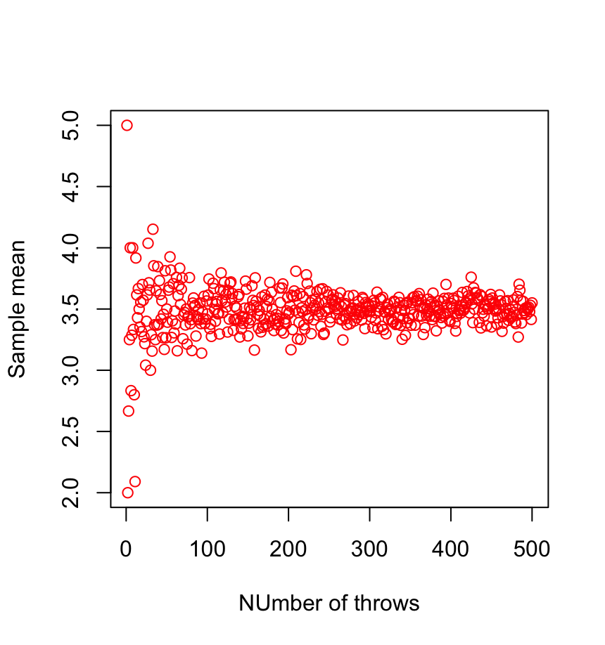
Consequence: a large number of i.i.d. subsystems can be described by very few parameters for \(N \gg 1\)
\(\Rightarrow\) e.g., a box with 1 mol of gas particles
Useful results from combinatorics
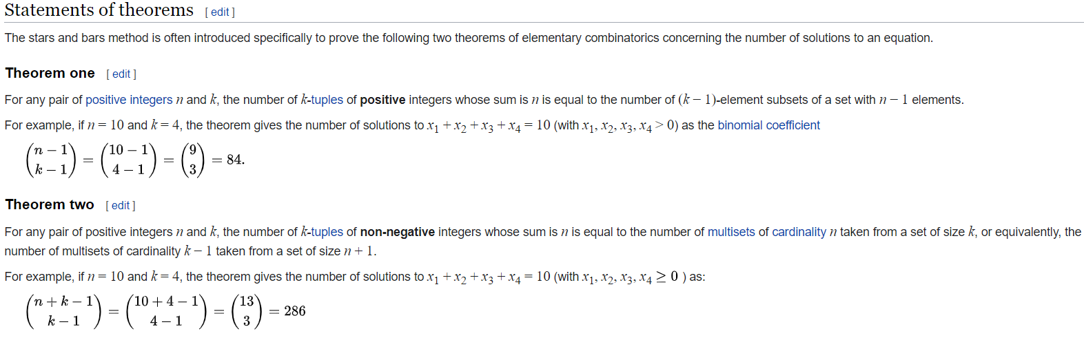
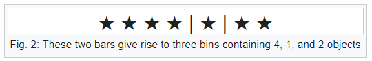
Bars & Stars theorems (|*)

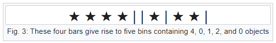
Emergence of statistical physics:
Coarse-graining
\(\bar{X}\)
Microstates, Mesostates and Macrostate
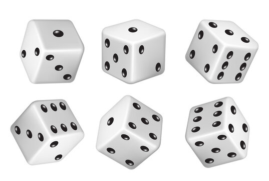
Consider a dice with 6 states
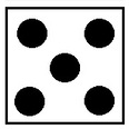
Let us throw a dice 5 times. The resulting sequence is
Microstate
The histogram of this sequence is
0
0
2
1
1
1
Mesostate
The average value is 3,8 Macrostate
Coarse-graining
Coarse-graining
# micro: \(6^5 =7776\)
# meso: \(\binom{6+5-1}{5} =252\)
# macro: \( 5\cdot 6-5\cdot 1 =25\)
Multiplicity W (sometimes \(\Omega\)):
# of microstates with the same mesostate/macrostate
Now we come back to the formula on Boltzmann's grave
Question: how do we calculate multiplicity W for mesostate
Answer: see combinatorics lecture.
Full answer: 1.) permute all states, 2.) take care of overcounting
1.) Permuation of all states: 5! = 120
2.) Overcounting - permutation of 2! = 2
Together: \(W(0,2,0,1,1,1) = \frac{5!}{2!} =60\)
0
0
2
1
1
1
Boltzmann-Gibbs-(Shannon) entropy
$$S = \log W \approx n\log n - n - \sum_{i} \left(n_i \log n_i - n_i \right)$$
Here, we use the normalization \(n = \sum_i n_i\)
and introduce probabilities \(p_i = n_i/n\)
$$ S = - n\sum_i p_i \log p_i$$
Finally the entropy per particle is
We use the Boltzmann formula (we set \(k_B = 1\) )
and Stirling's approximation \(\ln x! \approx x \ln x - x\)
We actually ended with the formula that is known as Shannon entropy in information theory
\( \mathcal{S} = S/n = -\sum_i p_i \log p_i \)
BGS entropy is a consequence of Boltzmann
By using the relation \(n_i/n = p_i\), we actually used the law of large numbers. It says that for large \(n\), the relative frequency of an event converges to its probability, i.e.,
\(p_i = \lim_{n \rightarrow \infty} \frac{n_i(n)}{n}\)
This limit is in physics called thermodynamic limit.
Law of large numbers
What is actually \(p_i\)?
0
0
1
1
1
2
P( )=1/3
Entropy in statistical physicds
- Suppose now that we make a measurement of our system
- In our example of 5 dice, we observe that the average value of a dice is \(\bar{X} = 3.8\) (i.e., the total sum is 19)
- We now ask, what is the mesostate that corresponds to this measurement
0
0
2
1
1
1
Possible mesostates:
0
1
2
0
1
1
How many mesostates are there?
0
0
1
0
4
0
etc.
Probability of a mesostate
- Here, the calculation is a bit more complicated since the (|*) theorem does not care that the maximum value on a dice is 6, so we have to exclude the cases that do not correspond to our example
- This can be solved by the so-called inclusion-exclusion principle, where we exclude unwanted cases
- After some algebra, the general formula gives us 17 distinct mesostates
We introduce the following notation:
0
0
1
1
1
\(=(6,5,4,2,2)\)
2
| (6,6,5,1,1) | (6,6,4,2,1) | (6,6,3,3,1) |
|---|---|---|
| (6,6,3,2,2) | (6,5,5,2,1) | (6,5,4,3,1) |
| (6,5,4,2,2) | (6,5,3,3,2) | (6,4,4,4,1) |
| (6,4,4,3,2) | (6,4,3,3,3) | (5,5,5,3,1) |
| (5,5,4,4,1) | (5,5,4,3,2) | (5,4,4,4,2) |
| (5,4,4,3,3) | (4,4,4,4,3) | (5,5,5,2,2) |
| (5,5,3,3,3) |
All mesostates with \(\bar{X} = 3.8\)
Q: What is the probability of observing such mesostate?
A: It is the multiplicity!
| W(6,6,5,1,1)=30 | W(6,6,4,2,1)=60 | W(6,6,3,3,1)=30 |
|---|---|---|
| W(6,6,3,2,2)=30 | W(6,5,5,2,1)=60 | W(6,5,4,3,1)=120 |
| W(6,5,4,2,2)=60 | W(6,5,3,3,2)=60 | W(6,4,4,4,1)=20 |
| W(6,4,4,3,2)=60 | W(6,4,3,3,3)=20 | W(5,5,5,3,1)=20 |
| W(5,5,4,4,1)=30 | W(5,5,4,3,2)=60 | W(5,4,4,4,2)=20 |
| W(5,4,4,3,3)=30 | W(4,4,4,4,3)=5 | W(5,5,5,2,2)=10 |
| W(5,5,3,3,3)=10 |
$$W(n_1,\dots,n_k) = \frac{n!}{n_1! n_2! \dots n_k!}$$
Probability of state with constraint
P( )
- How do we now calculate the probability of observing a value, e.g., what is ?
- For each mesostate, we calculate a probability of throwing three:
| P3(6,6,5,1,1)=0 | P3(6,6,4,2,1)=0 | P3(6,6,3,3,1)=0.4 |
|---|---|---|
| P3(6,6,3,2,2)=0.2 | P3(6,5,5,2,1)=0 | P3(6,5,4,3,1)=0.2 |
| P3(6,5,4,2,2)=0 | P3(6,5,3,3,2)=0.4 | P3(6,4,4,4,1)=0 |
| P3(6,4,4,3,2)=0.2 | P3(6,4,3,3,3)=0.6 | P3(5,5,5,3,1)=0.2 |
| P3(5,5,4,4,1)=0 | P3(5,5,4,3,2)=0.2 | P3(5,4,4,4,2)=0 |
| P3(5,4,4,3,3)=0.4 | P3(4,4,4,4,3)=0.2 | P3(5,5,5,2,2)=0 |
| P3(5,5,3,3,3)=0.6 |
Probability of state with constraint
- Now the probability is simply a weighted average of probabilities for each mesostate, weighted by its multiplicity, i.e.,
$$P(\qquad) = \frac{\sum_{m_i} P_3(m_i) W(m_i)}{\sum_{m_i} W(m_i)} = \frac{113}{605} \approx 18.7\%$$
here \(m_i\) are the mesostates that satisfy the constraint
This is quite complicated!
But what happens if we increase the number of dice?
Will it get more complicated or easier?
What happens if we rescale the problem?
- Suppose now that we do not throw 5 dice, but 10 dice, while the average value is the same (\(\bar{X} =3.8\)).
- What happens to multiplicity?
- Let us start with the mesostates, which are just double the mesostates for five dice, i.e., $$ (6,6,5,1,1) \mapsto (6,6,6,6,5,5,1,1,1,1)$$
- Then, the multiplicity can be expressed as
$$W(2n_1,\dots,2n_k) = \frac{(2n)!}{(2n_1)! (2n_2)! \dots (2n_k)!}$$
| W2(6,6,5,1,1)=3150 | W2(6,6,4,2,1)=12600 | W2(6,6,3,3,1)=6300 |
|---|---|---|
| W2(6,6,3,2,2)=3150 | W2(6,5,5,2,1)=12600 | W2(6,5,4,3,1)=113400 |
| W2(6,5,4,2,2)=12600 | W2(6,5,3,3,2)=12600 | W2(6,4,4,4,1)=420 |
| W2(6,4,4,3,2)=12600 | W2(6,4,3,3,3)=420 | W2(5,5,5,3,1)=420 |
| W2(5,5,4,4,1)=6300 | W2(5,5,4,3,2)=12600 | W2(5,4,4,4,2)=420 |
| W2(5,4,4,3,3)=3150 | W2(4,4,4,4,3)=45 | W2(5,5,5,2,2)=210 |
| W2(5,5,3,3,3)=210 |
Let us denote \(W_2(n_1,\dots,n_k) = W(2n_1,\dots,2n_k)\)
Multiplicities for double-configurations
What happens to the multiplicities?
Note: there are also other mesostates that are not double-configurations
Thermodynamic limit
- By rescaling the system, the most probable mesostates are observed much more often than the rest of the mesostates
- In thermodynamics, we are dealing with a large number of DOF (imagine \(10^{23}\) dice )
- As a consequence, only the mesostate with the largest multiplicity becomes relevant; all others become negligible
- How do we calculate the state with maximum multiplicity?
- We maximize the entropy (log of multiplicity) with respect to given constraints
Using Boltzmann's formula for non-multinomial systems
As we saw in the previous lecture, the multinomial multiplicity
$$W(n_1,\dots,n_k) = \binom{n}{n_1,\dots,n_k}$$
leads to Boltzmann-Gibbs-Shannon entropy.
$$S = - \sum_k p_k \log p_k$$
Are there systems with non-multinomial multiplicity?
What is their entropy?
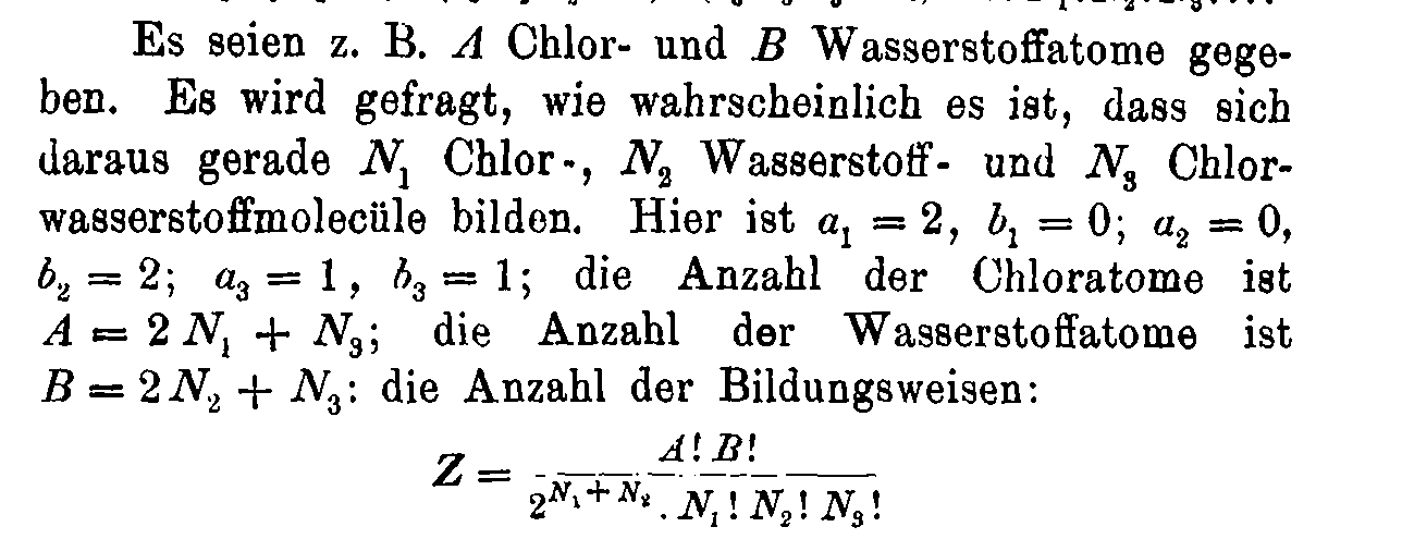
Ex. I: MB, FD & BE statistics
1. Maxwell-Boltzmann statistics - \(N\) distinguishable particles, \(N_i\) particles in state \(\epsilon_i\)
Multiplicity can be calculated as
$$W(N_1,\dots,N_k) = \binom{N}{N_1} \binom{N-N_1}{N_2} \dots \binom{N-\sum_{i=1}^{k-1}N_1}{N_k} = N! \prod_{i=1}^k \frac{1}{N_i!}$$
If \(\epsilon_i\) has degeneracy \(g_i\), then
$$W(N_1,\dots,N_k) = N! \prod_{i=1}^k \frac{g_i^{N_i}}{N_i!}$$
Then, we get
$$S_{MB} = - N \sum_{i=1}^k p_i \log \frac{p_i}{g_i}$$
Ex. I: MB, FD & BE statistics
2. Bose-Einstein statistics - \(N\) indistinguishable particles, \(N_i\) particles in state \(\epsilon_i\) with degeneracy \(g_i\),
Multiplicity can be calculated as
$$W(N_1,\dots,N_k) = \prod_{i=1}^k \binom{N_i + g_i-1}{N_i}$$
Let us introduce \(\alpha_i = g_i/N\). Then, we get
$$S_{BE} = N \sum_{i=1}^k \left[(\alpha_i + p_i) \log (\alpha_i +p_i) - \alpha_i \log \alpha_i - p_i \log p_i\right]$$
(|*)
3. Fermi-Dirac statistics - \(N\) indistinguishable particles, \(N_i\) particles in state \(\epsilon_i\) with degeneracy \(g_i\), maximally 1 particle per sub-level (thus \(N_i \leq g_i\))
Multiplicity can be calculated as
$$W(N_1,\dots,N_k) = \prod_{i=1}^k \binom{g_i}{N_i}$$
Let us introduce \(\alpha_i = g_i/N\). Then, we get
$$S_{FD} = N \sum_{i=1}^k \left[-(\alpha_i - p_i) \log (\alpha_i -p_i) + \alpha_i \log \alpha_i - p_i \log p_i\right]$$
Ex. I: MB, FD & BE statistics
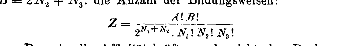
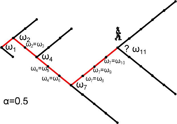
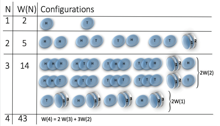
Ex. II: structure-forming systems
Let us start with a simple example of a coin tossing.
States are:


But! let's make a small change, we consider magnetic coins
The bound (or sticky) state is simply

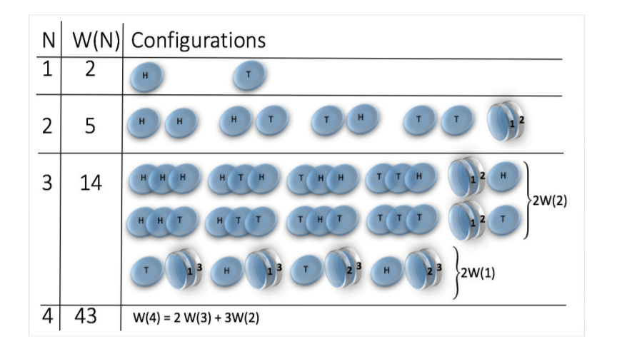
State space grows super-exponentially (\(W(n) \sim n^n \sim e^{n \log n}\) )
picture from: Jensen et al 2018 J. Phys. A: Math. Theor. 51 375002
Multiplicity


2 x 1x
1 x 1x
3
3
Microstate
Mesostate
Mesostate
2 x 1x
1 x 1x
1 1 2 2 3 3
2 3 1 3 1 2
3 2 3 1 2 1
1 1 2 2 3 3
2 3 1 3 1 2
3 2 3 1 2 1
= (1,2,3) , (2,1,3)
= (1,3,2) , (3,1,2)
= (2,3,1) , (3,2,1)
= (1,2,3) , (1,3,2)
= (2,1,3) , (2,3,1)
= (3,1,2) , (3,2,1)
How to calculate multiplicity
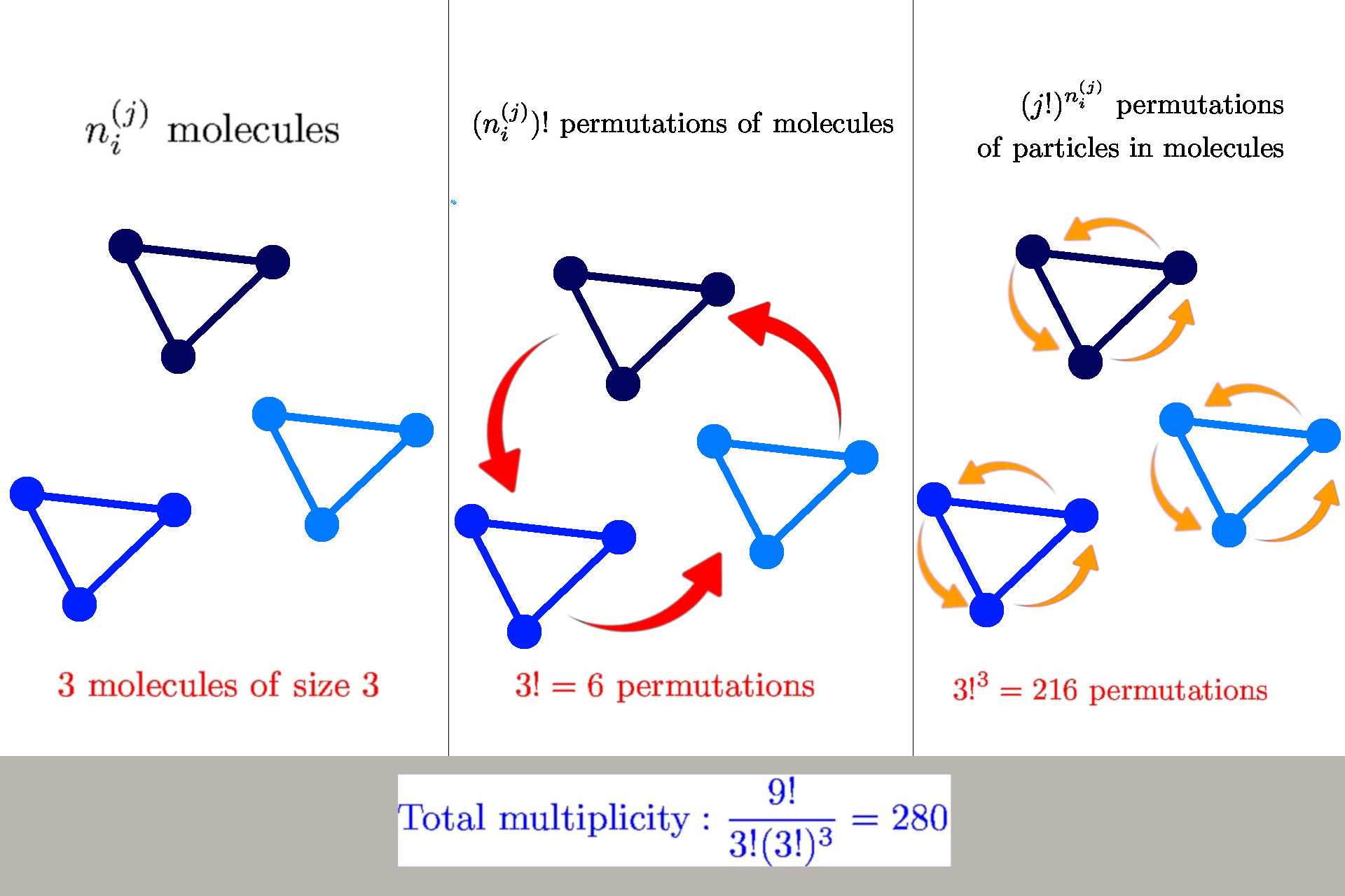
General formula: \(W(n_i^{(j)}) = \frac{n!}{\prod_{ij} n_i^{(j)}! {\color{red} (j!)^{n_i^{(j)}}}}\)
we have \(n_i^{(j)}\) molecules of size \(j\) in a state \(s_i^{(j)}\)
Multiplicity
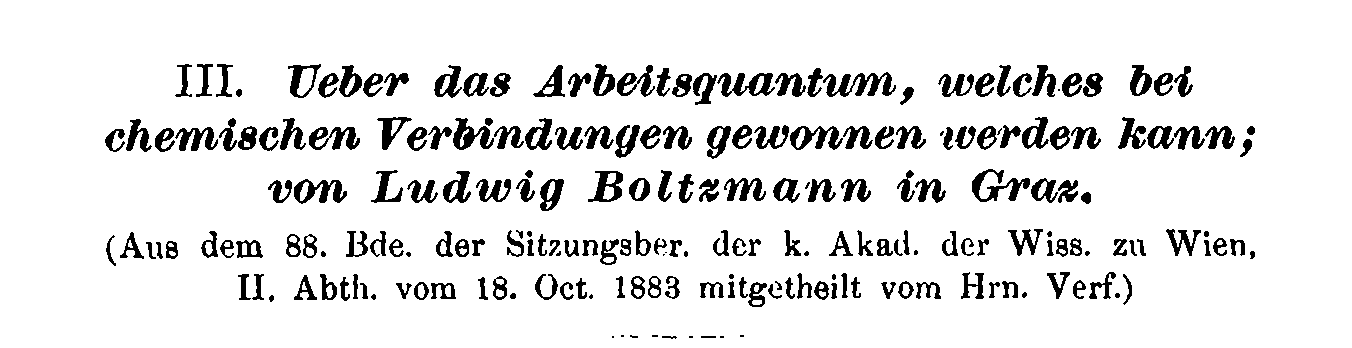
Boltzmann's 1884 paper
Entropy of structure-forming systems
$$ S = \log W \approx n \log n - \sum_{ij} \left(n_i^{(j)} \log n_i^{(j)} - n_i^{(j)} + {\color{red} n_i^{(j)} \log j!}\right)$$
Introduce "probabilities" \(\wp_i^{(j)} = n_i^{(j)}/n\)
$$\mathcal{S} = S/n = - \sum_{ij} \wp_i^{(j)} (\log \wp_i^{(j)} {\color{red}- 1}) {\color{red}- \sum_{ij} \wp_i^{(j)}\log \frac{j!}{n^{j-1}}}$$
Finite interaction range: concentration \(c = n/b\)
$$\mathcal{S} = S/n = - \sum_{ij} \wp_i^{(j)} (\log \wp_i^{(j)} {\color{red}- 1}) {\color{red}- \sum_{ij} \wp_i^{(j)}\log \frac{j!}{{\color{purple}c^{j-1}}}}$$
Nat. Comm. 12 (2021) 1127
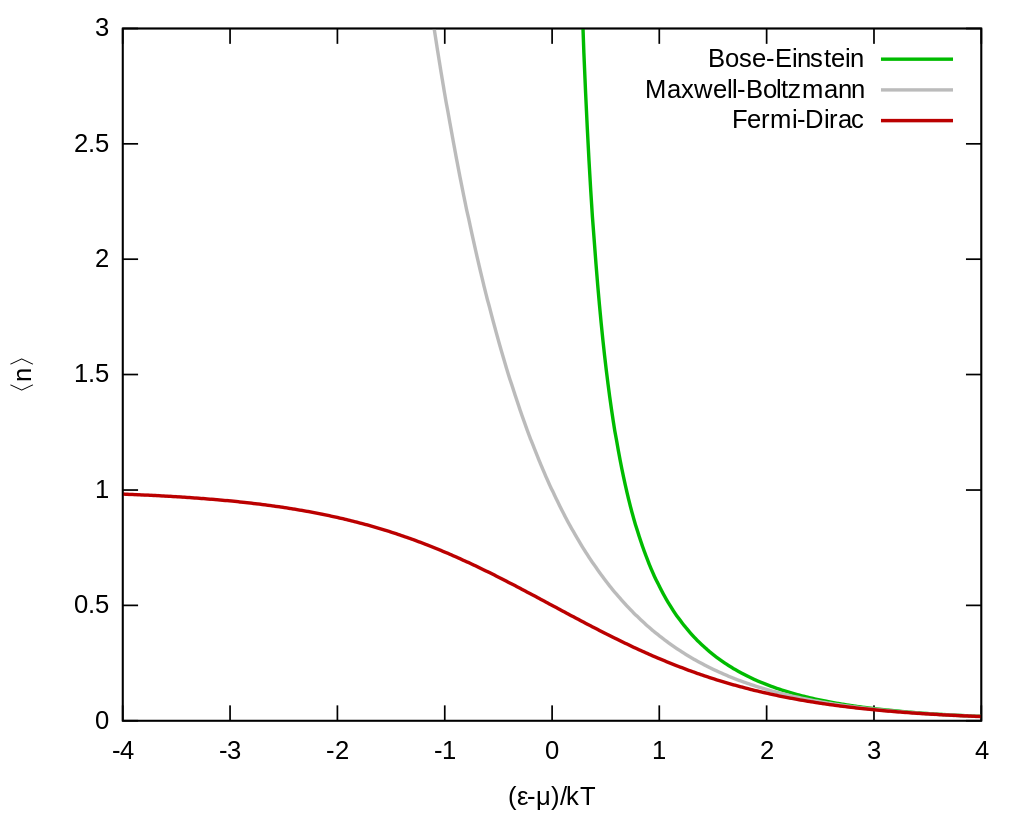
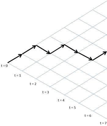
Ex. III: sample-space reducing processes (SSR)

Corominas Murtra, Hanel, Thurner PNAS 112(17) (2015) 5348

Multiplicity
The number of states is \(n\). Let us denote the states as \(x_n \rightarrow \dots \rightarrow x_1\), where \(x_1\) is the ground state, where the process restarts. Let us sample \(R\) relaxation sequences \(x = (x_{k_1},\dots,x_1)\).
The sequences can be visualised as
How many of these sequences contain a state \(x_{j}\) exactly \(k_j\) times?

Each run must contain \(x_1\)
Multiplicity
Number or runs \(R \equiv k_1\), number of them containing \(x_j\) is \(k_j\)
Multiplicity of these sequences: \(\binom{k_1}{k_j}\)
By multiplying the multiplicity for each state we get
$$W(k_1,\dots,k_n) = \prod_{j=2}^n \binom{k_1}{k_j}$$
$$ \log W \approx \sum_{j=2}^n \left[k_1 \log k_1 - \cancel{k_1} - k_j \log k_j + \cancel{k_j} - (k_1-k_j) \log (k_1 - k_j) + \cancel{(k_1-k_j)}\right]$$
$$\approx \sum_{j=2}^n \left[ k_1 \log k_1 \textcolor{red}{-k_j \log k_1} - k_j log \frac{k_j}{\textcolor{red}{k_1}} - (k_1-k_j) \log(k_1-k_j) \right]$$
By introducing \(p_i = k_i/N\) where \(N\) is the total number of steps, we get
$$S_{SSR}(p) = - N \sum_{j=2}^n \left[p_i \log \left(\frac{p_i}{p_1}\right) + (p_1-p_i) \log \left(1-\frac{p_i}{p_1}\right)\right]$$
Ex. IV: Pólya urns

Hanel, Corominas Murtra, Thurner New J. Phys. (2017) 19 033008
Probability of a sequence
We have \(c\) colors, initially \(n_i(0) \equiv n_i\) balls of color \(c_i\). After a ball is drawn, we return \(\delta\) balls of the same color to the urn.
After \(N\) draws, the number of balls in the urn is
$$n_i(N) = n_i + \delta k_i$$
where \(k_i\) is the number of draws of color \(c_i\). The total number of balls is \(n(R) = \sum_{c} n_c(N) = N + \delta N\)
The probability of drawing a ball of color \(c_i\) in \(N\)-th run, is \(p_i(N) = n_i(N)/n(N)\). The probability of sequence
\(\ \mathcal{I} =\{i_1,\dots,i_N\} \) is
$$p(\mathcal{I}) = \prod_{j=1}^c \frac{n_{j}^{(\delta,k_j)}}{n^{(\delta,N)}}$$
where \(m^{(\delta,r)} = m(m+\delta)\dots(m+r\delta)\)
Probability of a histogram
A histogram \(\mathcal{K} = \{k_1,\dots,k_c\}\) is defined as \(k_c = \sum_{j = 1}^N \delta(i_j,c) \)
Thus the probability of observing a histogram is
$$ p(\mathcal{K}) = \binom{N}{k_1,\dots,k_c} p(\mathcal{I}) $$
\(n_{j}^{(\delta,k_{j})} \approx k_{j}! \delta^{k_{j}} (k_i+1)^{n_i/\delta} \)
\( p(\mathcal{K}) = \frac{N!}{\prod_{j=1}^c \cancel{k_j!}} \frac{\prod_{j=1}^c \cancel{k_j!} \delta^{k_j} (k_j+1)^{n_j/\delta}}{n^{(\delta,N)}} \)
... technical calculation ...
$$S_{Pólya}(p) = \log p(\mathcal{K}) \approx - \sum_{i=1}^c \log(p_i + 1/N)$$
Ex. IV: q-deformations
This example is rather theoretical, but provides us a useful hint of what happens if there are correlations in the sample space
Motivation: finite versions of \(\exp\) and \(\log\)
\(\exp(x) = \lim_{n \rightarrow \infty} \left(1+\frac{x}{n}\right)^n\)
So define
\(\exp_q(x) := \left(1 + (1-q) x\right)^{1/(1-q)}\)
\(\log_q(x) := \frac{x^{1-q}-1}{1-q}\)
Let us find an operation s.t.
\(\exp_q(x) \otimes_q \exp_q(y) \equiv \exp_q(x+y)\)
\(\Rightarrow a \otimes_q b = \left[a^{1-q} + b^{1-q}-1\right]^{1/(1-q)}\)
Suyari, Physica A 368 (2006) 63-82
Calculus of q-deformations
In analogy to \(n! = 1 \cdot 2 \cdot \dots \cdot n\) introduce \(n!_q := 1 \otimes_q 2 \otimes_q \dots \otimes_q n\)
It is than easy to show that \(\log_q n!_q = \frac{\sum_{k=1}^n k^{1-q} - n}{1-q}\) which can be used for generalized Stirling's approximation \(\log_q n!_q \approx \frac{n}{2-q} \log_q n\)
Let us now consider a q-deformed multinomial factor
$$\binom{n}{n_1,\dots,n_k}_q := n!_q \oslash_q (n_1!_q \otimes_q \dots \otimes_q n_k!_q) $$
$$ = \left[\sum_{l=1}^n l^{1-q} - \sum_{i_1}^{n_1} i_i^{1-q} - \dots - \sum_{i_k}^{n_k} i_k^{1-q}\right]^{1/(1-q)}$$
Tsallis entropy
Let us consider that the multiplicity is given by a q-multinomial factor \( W(n_1,\dots,n_k) = \binom{n}{n_1,\dots,n_k}_q\)
In this case, it is more convenient to define entropy as \(S = \log_q W\), which gives us:
$$\log_q W = \frac{n^{2-q}}{2-q} \frac{\sum_{i=1}^k p_i^{2-q}-1}{q-1} = \frac{n^{2-q}}{2-q} S_{2-q}(p)$$
This entropy is known as Tsallis entropy
Note that the prefactor is not \(n\) but \(n^{2-q}\)
(non-extensivity) - we will discuss this later
Entropy and energy
Until now, we have been just counting states; let us now discuss the relation with energy.
We consider that the states describe the energy of the system (either Hamiltonian or more generalized energy functional)
Therefore, entropy is defined as
$$ S(E) := \log W(E)$$
Ensembles
There are a few typical situations:
1. Isolated system = microcanonical ensemble
Let \(H(s)\) be the energy of a state \(s\). Multiplicity is then \(W(E) = \sum_{s} \delta(H(s) - E)\)
Phenomena like negative "temperature" \(T = \frac{\mathrm{d} S(E)}{\mathrm{d} E} < 0\)
2. closed system = canonical ensemble
Total system is composed of the system of interest (S) and the heat reservoir/bath (B). They are weakly coupled i.e., \(H_{tot}(s,b) = H_S(s) + H_B(b)\) (no interaction energy)
$$W(E_{tot}) = \sum_{s,b} \delta(H_{tot}(s,b) -E_{tot})$$
3. open system = grandcanonical ensemble
This can be further rewritten as
$$= \int \mathrm{d} E_S\, \sum_s \delta (H_{S}(s)-E_S) \sum_b(H_B(b)-(E_{tot}-E_S)) $$
$$= \int \mathrm{d} E_S \, W_S(E_S) W_B(E_{tot}-E_S) $$
Entropy in canonical ensemble
This is hard to calculate. Typically, the dominant contribution is from the maximal configuration of the integrand, which we obtain from
$$\frac{\partial W_S(E_S) W_B(E_{tot}-E_S)}{\partial E_S} \stackrel{!}{=} 0 \Rightarrow \frac{W'_S(E_S)}{W_S(E)} = \frac{W'_B(E_{tot}-E_S)}{W_B(E_{tot}-E_S)}$$
As a consequence \(\frac{\partial S_E(E_S)}{\partial E_S} \stackrel{!}{=} \frac{\partial S_B(E_{tot}-E_S)}{\partial E_S} := \frac{1}{k_B T}\)
and \(\underbrace{S_B(E_{tot} - E_S)}_{free \ entropy} = \underbrace{S_B(E_{tot})}_{bath \ entropy} - \frac{\partial S}{\partial E_S} E_S + \dots\)
This is the emergence of Maximum entropy principle
Canonical ensemble & Coarse-graining
S
B
weak coupling
S
coarse-graining
Deterministic picture
Statistical
picture
Maximum entropy principle
General approach - method of Lagrange multipliers
Maximize \(L(p) = S(p) - \alpha \sum_i p_i - \sum_k \lambda_k \sum_i I_{i,k} p_i\)
$$\frac{\partial L}{\partial p_i} = \frac{\partial S(p)}{\partial p_i} - \alpha - \sum_k \lambda_k I_{i,k} \stackrel{!}{=} 0$$
In case \(\psi_i(P) = \frac{\partial S(p)}{\partial p_i}\) is invertible for \(p_i\), we get that
$$ p^{\star}_i = \psi_i^{(-1)}\left(\alpha + \sum_k \lambda_k I_{i,k}\right)$$
Legendre structure of thermodynamics - interpretation of L
$$L(p) = S(p) - \beta U(p) = \Psi(p) = - \beta F(p)$$
free entropy
MB, BE & FD MaxEnt
Maxwell-Boltzmann
\(S_{MB} = - \sum_{i=1}^k p_i \log \frac{p_i}{g_i}\)
\(p_i^\star = \frac{g_i}{Z} \exp(-\epsilon_i/ T) \)
Bose-Einstein
\(S_{BE} = \sum_{i=1}^k \left[(\alpha_i + p_i) \log (\alpha_i +p_i) - \alpha_i \log \alpha_i - p_i \log p_i\right]\)
\(p_i^\star = \frac{\alpha_i}{Z} \frac{1}{\exp(\epsilon_i/ T)-1} \)
Fermi-Dirac
\(S_{FD} = \sum_{i=1}^k \left[-(\alpha_i - p_i) \log (\alpha_i -p_i) + \alpha_i \log \alpha_i - p_i \log p_i\right]\)
\(p_i^\star = \frac{\alpha_i}{Z} \frac{1}{\exp(\epsilon_i/ T)+1} \)
Slide title
MB, BE & FD MaxEnt
Structure-forming systems
$$S(\wp) =- \sum_{ij} \wp_i^{(j)} (\log \wp_i^{(j)} - 1) - \sum_{ij} \wp_{ij} \log \frac{j!}{n^{j-1}}$$
Normalization: \(\sum_{ij} j \wp_{i}^{(j)} =1 \) Energy: \(\sum_{ij} \epsilon_{i}^{(j)} \wp_{i}^{(j)} = U\)
where \( j \wp_i^{(j)} = p_i^{(j)}\)
MaxEnt distribution: \(\wp_i^{(j)} = \frac{n^{j-1}}{j!} \exp(-\alpha j -\beta \epsilon_i^{(j)})\)
The normalization condition gives \(\sum_j j \mathcal{Z}_j e^{-\alpha j} = 1 \)
where \(\mathcal{Z}_j = \frac{n^{j-1}}{j!} \sum_i \exp(-\beta \epsilon_i^{(j)}) \) is the partial partition function
We get a polynomial equation in \(e^{-\alpha}\)
Average number of molecules \(\mathcal{M} = \sum_{ij} \wp_{i}^{(j)}\)
Free energy: \(F = U - T S = -\frac{\alpha}{\beta} - \frac{\mathcal{M}}{\beta} \)
MaxEnt of Tsallis entropy
$$S_q(p) = \frac{\sum_i p_i^q-1}{1-q}$$
MaxEnt distribution is: \(p_i^\star = \exp_q(\alpha+\beta \epsilon_i)\)
Note that this is not equal in general to \(q_i^\star =\frac{\exp_q(\beta \epsilon_i)}{\sum_i \exp_q( \beta \epsilon_i)}\)
However, it is possible to use the identity
$$\exp_q(x+y) = \exp_q(x) \exp_q\left(\frac{y}{\exp_q(x))^{1-q}}\right)$$
The MaxEnt distribution of Tsallis entropy can be expressed as
$$p_i^\star(\beta) = \exp_q(\alpha+\beta \epsilon_i) = \exp_q(\alpha) \exp_q(\tilde{\beta}\epsilon_i) = q_i^\star(\tilde{\beta}) $$
where \( \tilde{\beta} = \frac{\beta}{\exp_q(\alpha)^{1-q}}\)
(sometimes called self-referential temperature)
MaxEnt for path-dependent processes
and relative entropy
- What is the most probable histogram of a process \(X(N,\theta)\)?
- \(\theta\) - parameters, \(k\) histogram of \(X(N,\theta) \)
- \(P(k|\theta)\) is probability of finding a histogram
- Most probable histogram \(k^\star = \argmin_k P(k|\theta) \)
-
In many cases, the probability can be decomposed to $$P(k|\theta) = W(k) G(k|\theta)$$
- \(W(k)\) - multiplicity of histogram
- \(G(k|\theta)\) - probability of a microstate belong to \(k\)
-
$$\underbrace{\log P(k|\theta)}_{S_{rel}}= \underbrace{\log W(k)}_{S_{MEP}} + \underbrace{\log G(k|\theta)}_{S_{cross}} $$
- \(S_{rel}\) - relative entropy (divergence)
- \(S_{cross}\)- cross-entropy, depends on constraints given by \(\theta\)
The role of constraints
The cross-entropy corresponds to the constraints
For the case of expected energy, it can be expressed through the cross entropy
$$S_{cross}(p|q) = - \sum_i p_i \log q_i $$
where \(q_i\) are prior probabilities. By taking \(q^\star_i = \frac{1}{Z}e^{-\beta \epsilon_i}\) we get
$$S_{cross}(p|q^\star) = \beta\sum_i p_i \epsilon_i + \ln Z$$
However, for the case of path-dependent process, the natural constraints might not be of this form
Kullback-Leibler divergence
$$D_{KL}(p||q) = -S(p) + S_{cross}(p,q) $$
$$S_{SSR}(p) = - N \sum_{j=2}^n \left[p_i \log \left(\frac{p_i}{p_1}\right) + (p_1-p_i) \log \left(1-\frac{p_i}{p_1}\right)\right]$$
MaxEnt for SSR processes
From multiplicity of trajectory histograms, we have shown that the entropy of SSR is
Let us now consider that after each run (when the system reaches the ground state) we drive the ball to a random state with probability \(q_i\)
After each jump the effective space reduces
MaxEnt for SSR processes
One can see that the probability of sampling a histogram \(k_i\) is
$$G(k|q) = \prod_{i=1}^n \frac{q_i^{k_i}}{Q_{i-1}^{k_i}} $$
where \(Q_i = \sum_{j=1}^i q_i\) and \(Q_0 \equiv 1\).
$$S_{cross}(p|q) = - \sum_{i=1}^n p_i \log q_i - \sum_{i=2}^n p_i \log Q_{i-1} $$
By assuming in \(q_i \propto e^{-\beta \epsilon_i}\) the cross-entropy is
$$S_{cross}(p|q) = \beta \sum_{i=1}^n p_i \epsilon_i + \beta \sum_{i=2}^n p_i f_i = \mathcal{E} + \mathcal{F}$$
where \(f_i = \ln \sum_i e^{-\beta \epsilon_i}\)
MaxEnt for Pólya urns
Probability of observing a histogram
$$ p(\mathcal{K}) = \binom{N}{k_1,\dots,k_c} p(\mathcal{I}) $$
By carefully taking into account the initial number of balls in the urn \(n_i\) we end with
$$S_{Pólya}(p) = - \sum_{i=1}^c \log(p_i + 1/N)$$
$$S_{Pólya}(p|q) = - \sum_{i=1}^c \left[\frac{q_i}{\gamma} \log \left(p_i + \frac{1}{N}\right) - \log\left(1+\frac{1}{N\gamma} \frac{q_i - \gamma}{p_i+\frac{1}{N}}\right)+ \log q_i\right]$$
where \(q_i = n_i/N, \gamma=\delta/N\)
Long-run limit
$$S_{Pólya}(p) = - \sum_{i=1}^c \log p_i$$
$$S_{Pólya}(p|q) = - \sum_{i=1}^c \left[\frac{q_i}{\gamma} \log p_i + \log q_i\right]$$
By taking \(N \rightarrow \infty\), we get
with some assumptions for p and q
Related extremization principles
As we already found out, the MaxEnt principle can be seen as a special case of the principle of minimum relative entropy
$$p^\star = \arg\min_p D(p||q)$$
In many cases, the divergence can be expressed as \(D(p||q) = - S(p) + S_{cross}(p,q)\)
It connects information theory, thermodynamics and geometry
Priors \(q\) can be obtained from theoretical models or measurements
Posteriors \(p\) can be from parametric family or from a special class of probability distributions
Relative entropy is well defined for both discrete and continuous distributions
Maximization for trajectory probabilities - Maximum caliber
Let us now consider the whole trajectory \(\pmb{x}(t)\) with probability \(p(\pmb{x}(t))\)
We define the term caliber, which is the KL-divergence of the path probability
$$S_{cal}(p|q) = \int \mathcal{D} \pmb{x}(t) p(\pmb{x}) \log \frac{p(\pmb{x}(t))}{q(\pmb{x}(t))}$$
N.B.: Entropy production can be written in terms of caliber as
$$\Sigma_t = S_{cal}[p(\pmb{x}(t))|\tilde{p}(\tilde{\pmb{x}}(t))]$$
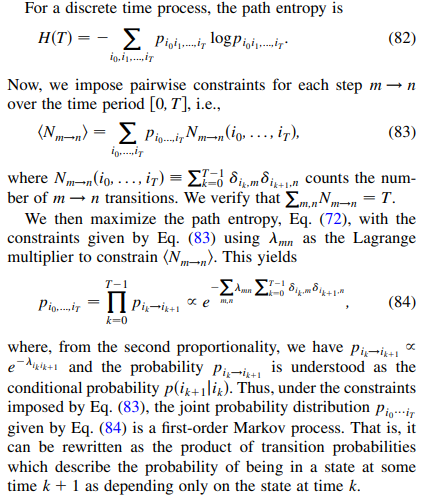
MaxCal and Markov processes
Axiomatic approaches
Now we do the opposite approach compared to lecture II.
We postulate the properties we think entropy should have
and derive the corresponding entropic funcional
These axiomatic approaches have different nature, we will discuss their possible connection
- Continuity.—Entropy is a continuous function of the probability distribution only.
- Maximality.— Entropy is maximal for the uniform distribution.
- Expandability.— Adding an event with zero probability does not change the entropy.
- Additivity.— \(S(A \cup B) = S(A) + S(B|A)\) where \(S(B|A) = \sum_i p_i^A S(B|A=a_i)\)
Shannon-Khinchin axioms
Introduced independently by Shannon and Khinchin
Motivated by information theory
These four axioms uniquely determine Shannon entropy
\(S(P) = - \sum_i p_i \log p_i\)
SK axioms serve as a starting point for other axiomatic schemes
Non-additive SK axioms
Several axiomatic schemes generalize axiom SK4.
One possibility is to generalize additivity. The most prominent example is q-additivity
$$ S(A \cup B) = S(A) \oplus_q S(B|A)$$
where \(x \oplus_q y = x + y + (1-q) xy\) is q-addition
\(S(B|A)= \sum_i \rho_i(q)^A S(B|A=a_i)\) is conditional entropy
and \(\rho_i = p_i^q/\sum_k p_k^q\) is escort distribution.
This uniquely determines Tsallis entropy
$$S_q(p) = \frac{1}{1-q}\left(\sum_i p_i^q-1\right)$$
Abe, Phys. Lett. A 271 (2000) 74.
Kolmogorov-Nagumo average
Another possibility is to consider a different type of averaging
In the original SK axioms, the conditional entropy is defined as the arithmetic average of \(S(B|A=a_i)\)
We can use alternative averaging, as Kolmogoro-Nagumo average
$$\langle X \rangle_f = f^{-1} \left(\sum_i p_i f(x_i)\right)$$
By keeping addivity, but taking \(S(B|A)= f^{-1}(\sum_i \rho_i(q)^A f(S(B|A=a_i))\)
for \(f(x) = \frac{e^{(1-q)x}-1}{1-q}\) we uniquely obtain Rényi entropy
$$R_q(p) = \frac{1}{1-q}\log \sum_i p_i^q$$
Jizba, Arimitsu, Annals of Physics 312 (1) (2004)17-59
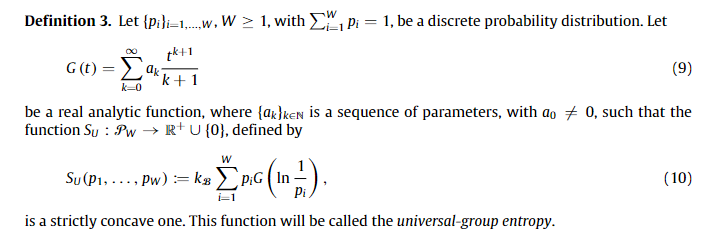
Entropy composability
and group entropies
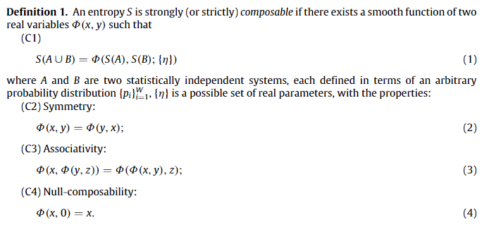
Entropy composability
and group entropies
- Axiomatization from the Maximum entropy principle point of view
- Principle of maximum entropy is an inference method and it should obey some statistical consistency requirements.
- Shore and Johnson set the consistency requirements:
- Uniqueness.—The result should be unique.
- Permutation invariance.—The permutation of states should not matter.
- Subset independence.—It should not matter whether one treats disjoint subsets of system states in terms of separate conditional distributions or in terms of the full distribution.
- System independence.—It should not matter whether one accounts for independent constraints related to disjoint subsystems separately in terms of marginal distributions or in terms of full-system constraints and joint distribution.
- Maximality.—In absence of any prior information the uniform distribution should be the solution.
Shore-Johnson axioms
P.J., J.K. Phys. Rev. Lett. 122 (2019), 120601
Shannon & Khinchin meet Shore & Johnson
Are the axioms set by theory of information and statistical inference different or can we find some overlap?
Let us consider the 4th SK axiom
in the form equivalent to composability axiom by P. Tempesta:
4. \(S(A \cup B) = f[f^{-1}(S(A)) \cdot f^{-1}(S(B|A))]\)
\(S(B|A) = S(B)\) if B is independent of A.
Entropies fulfilling SK and SJ: $$S_q^f(P) = f\left[\left(\sum_i p_i^q\right)^{1/(1-q)}\right] = f\left[\exp_q\left( \sum_i p_i \log_q(1/p_i) \right)\right]$$
Phys. Rev. E 101, 042126 (2020)
Lieb-Yngvason axioms
Lieb and Yngvason define thermodynamics via adiabatic accessibility following axioms:
- A1 (Reflexivity): For any state \(X\), \(X \prec X\).
- A2 (Transitivity): If \(X \prec Y\) and \(Y \prec Z\), then \(X \prec Z\).
- A3 (Consistency): If \(X \prec X'\) and \(Y \prec Y'\), then \((X,Y) \prec (X',Y')\)
- A4 (Scaling Invariance): If \(X \prec Y\), then \(\lambda X \prec \lambda Y\) for all \(\lambda > 0\)
- A5 (Splitting and Recombination): For \(0 < \lambda < 1\),
$$X \sim (\lambda X, (1-\lambda)X)$$
- A6 (Stability): If \((X, \epsilon Z) \prec (Y, \epsilon Z)\) for a sequence \(\epsilon \to 0\), then \(X \prec Y\).
Lieb-Yngvason axioms
Entropy in LY framework should fulfill these axioms
- (E1) Monotonicity:
\(X \prec Y \;\Longleftrightarrow\; S(X) \le S(Y)\) - (E2) Additivity:
\(S(X,Y) = S(X) + S(Y)\) - (E3) Extensivity:
\(S(\lambda X) = \lambda S(X), \quad \text{for all } \lambda > 0.\)
Boltzmann entropy & Lieb-Yngvason axioms
Does BE satisfy LY axioms?
- (E1) Monotonicity:
- In standard settings, yes (H-theorem)
- (E2) Additivity:
yes: \(W(X,Y) = W(X)\,W(Y)\;\;\Rightarrow\;\;S_B(X,Y) = S_B(X) + S_B(Y)\) - (E3) Extensivity:
yes, for short-range interactions: \(W(\lambda X) \sim [W(X)]^\lambda \;\; \Rightarrow \;\; S_B(\lambda X) = \lambda S_B(X),\)
Appropriate for ''simple'' systems
Entropy and scaling
We have been mentioning the issue of extensivity before
Let us see how the multiplicity and entropy scales with size \(N\)
This allows us to introduce a classification of entropies
- How does the sample space change when we rescale its size \( N \mapsto \lambda N \)?
- If the ratio behaves like \(\frac{W(\lambda N)}{W(N)} \sim \lambda^{c_0} \) for \(N \rightarrow \infty\), the exponent can be extracted by \(\frac{d}{d\lambda}|_{\lambda=1}\): \(c_0 = \lim_{\rightarrow \infty} \frac{N W'(N)}{W(N)}\)
- For the leading term we have \(W(N) \sim N^{c_0}\).
- Let us use the other rescaling \( N \mapsto N^\lambda \)
- The we get that \(\frac{W(N^\lambda)}{W(N)} \frac{N^{c_0}}{N^{\lambda c_0}} \sim \lambda^{c_1}\)
- First correction is \(W(N) \sim N^{c_0} (\log N)^{c_1}\)
Multiplicity scaling
-
We define the set of rescalings \(r_\lambda^{(n)}(x) := \exp^{(n)}(\lambda \log^{(n)}(x) \) )
- \( f^{(n)}(x) = \underbrace{f(f(\dots(f(x))\dots))}_{n \ times}\)
- \(r_\lambda^{(0)}(x) = \lambda x\), \(r_\lambda^{(1)}(x) = x^\lambda\), \(r_\lambda^{(2)}(x) = e^{\log(x)^\lambda} \), ...
- They form a group: \(r_\lambda^{(n)} \left(r_{\lambda'}^{(n)}\right) = r_{\lambda \lambda'}^{(n)} \), \( \left(r_\lambda^{(n)}\right)^{-1} = r_{1/\lambda}^{(n)} \), \(r_1^{(n)}(x) = x\)
-
We repeat the procedure: \(\frac{W(N^\lambda)}{W(N)} \frac{N^{c_0} (\log N)^{c_1} }{N^{\lambda c_0} (\log N^\lambda)^{c_1}} \sim 1\),
- We take \(N \mapsto r_\lambda^{(2)}(N)\)
- \(\frac{W(r_\lambda^{(2)}(N))}{W(N)} \frac{N^{c_0} (\log N)^{c_1} }{r_\lambda^{(2)}(N)^{c_0} (\log r_\lambda^{(2)}(N))^{c_1}} \sim \lambda^{c_2}\),
- Second correction is \(W(N) \sim N^{c_0} (\log N)^{c_1} (\log \log N)^{c_2}\)
Multiplicity scaling
- General correction \( \frac{W(r_\lambda^{(k)}(N))}{W(N)} \prod_{j=0}^{k-1} \left(\frac{\log^{(j)} N}{\log^{(j)}(r_\lambda^{(k)}(N))}\right)^{c_j} \sim \lambda^{\bf c_k}\)
- Possible issue: what if \(c_0 = +\infty\)? \(W(N)\) grows faster than any \(N^\alpha\)
- We replace \(W(N) \mapsto \log W(N)\)
- The leading order scaling is \(\frac{\log W(\lambda N)}{\log W(N)} \sim \lambda^{c_0} \) for \(N \rightarrow \infty\)
- So we have \(W(N) \sim \exp(N^{c_0})\)
- If this is not enough, we replace \(W(N) \mapsto \log^{(l)} W(N)\) so that we get finite \(c_0\)
- General expansion of \(W(N)\) is $$W(N) \sim \exp^{(l)} \left(N^{c_0}(\log N)^{c_1} (\log \log N)^{c_2} \dots\right) $$
J.K., R.H., S.T. New J. Phys. 20 (2018) 093007
Multiplicity scaling
Extensive entropy
- We can do the same procedure with entropy \(S(W)\)
- Leading order scaling: \( \frac{S(\lambda W)}{S(W)} \sim \lambda^{d_0}\)
-
First correction \( \frac{S(W^\lambda)}{S(W)} \frac{W^{d_0}}{W^{\lambda d_0}} \sim \lambda^{d_1}\)
- First two scalings correspond to \((c,d)\)-entropy for \(c= 1-d_0\) and \(d = d_1\)
- Scaling expansion of entropy $$S(W) \sim W^{d_0} (\log W)^{d_1} (\log \log W)^{d_2} \dots $$
-
Requirement of extensivity \(S(W(N)) \sim N\) determines the relation between \(c\) and \(d\) :
- \(d_l = 1/c_0\), \(d_{l+k} = - c_k/c_0\) for \(k = 1,2,\dots\)
| Process | S(W) | |||
|---|---|---|---|---|
| Random walk |
0 |
1 |
0 |
|
| Aging random walk |
0 |
2 |
0 |
|
| Magnetic coins * |
0 |
1 |
-1 |
|
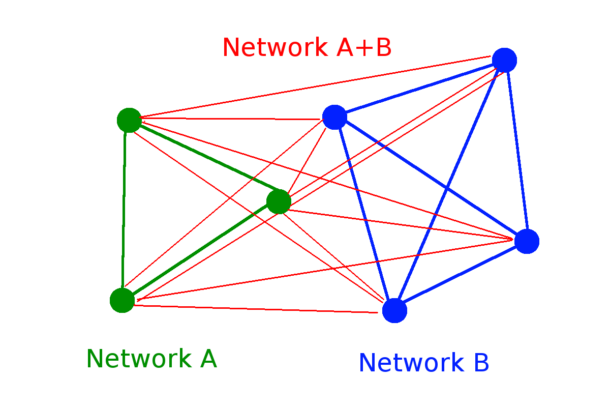
| Random network |
0 |
1/2 |
0 |
|
| Random walk cascade |
0 |
0 |
1 |
\( \log W\)
\( (\log W)^2\)
\( (\log W)^{1/2}\)
\( \log \log W\)
\(d_0\)
\(d_1\)
\(d_2\)
\( \log W/\log \log W\)
* H. Jensen et al. J. Phys. A: Math. Theor. 51 375002
\( W(N) = 2^N\)
\(W(N) \approx 2^{\sqrt{N}/2} \sim 2^{N^{1/2}}\)
\( W(N) \approx N^{N/2} e^{2 \sqrt{N}} \sim e^{N \log N}\)
\(W(N) = 2^{\binom{N}{2}} \sim 2^{N^2}\)
\(W(N) = 2^{2^N}-1 \sim 2^{2^N}\)

Parameter space of \( (c,d) \) entropy
How does it change for one more scaling exponent?
R.H., S.T. EPL 93 (2011) 20006
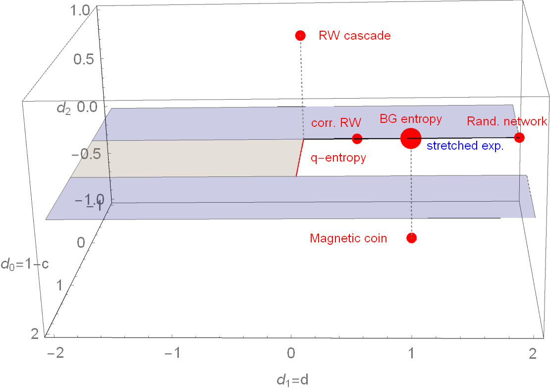
Parameter space of \( (d_0,d_1,d_2) \)-entropy
To fulfill SK axiom 2 (maximality): \(d_l > 0\), to fulfill SK axiom 3 (expandability): \(d_0 < 1\)
Thank you for your attention
csh.ac.at
Foundations of entropy in complex systems - Ising Lecture 2026
By Jan Korbel


