Thermodynamics of structure-forming systems

Jan Korbel

Slides available at: slides.com/jankorbel

Personal web: jankorbel.eu

JETC 2025, Belgrade

Structure-forming systems

• Many real-world systems form structures:
  • molecules of atoms
  • clusters of colloidal particles
  • (bio)polymers or micelles
  • social groups
• The main characteristic is that the number of structures (e.g., molecules) is not conserved, while the number of entities (e.g., particles) is conserved

Grand-canonical ensemble

• These systems are typically described by the grand-canonical ensemble with chemical potential(s) \(\mu_i\)
• The particle conservation is obeyed only on average by using the mass action law
• In chemistry, we are dealing with large systems 
• What if the system consists of a small number of particles?
• But is it possible to describe the systems with the canonical ensemble? 

Thermodynamics of structure-forming systems

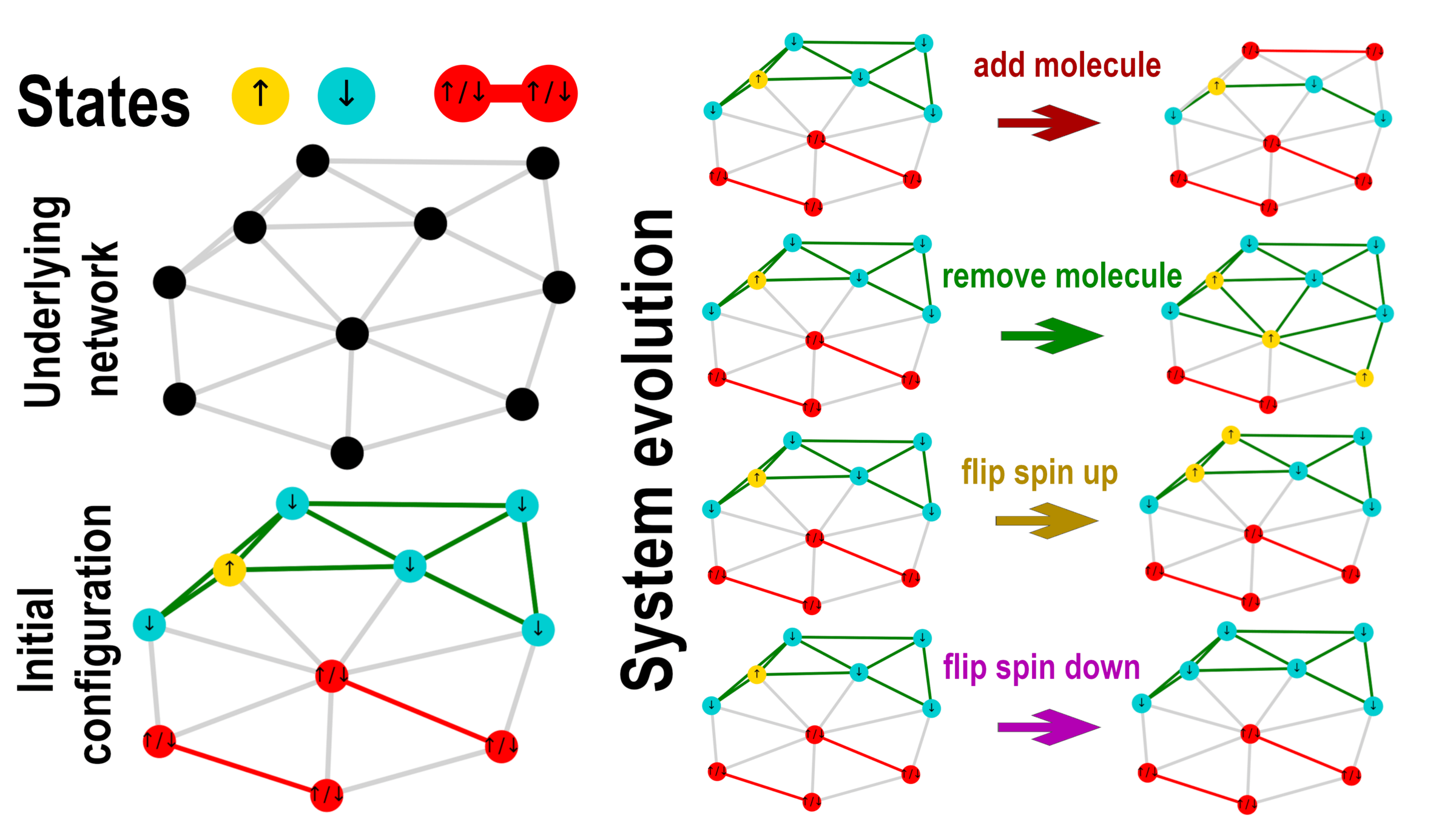
Toy model - magnetic coin model

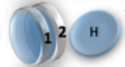
We consider a coin with two states: head             and tail

The coins are magnetic and can stick together 

How many states we get for N coins?

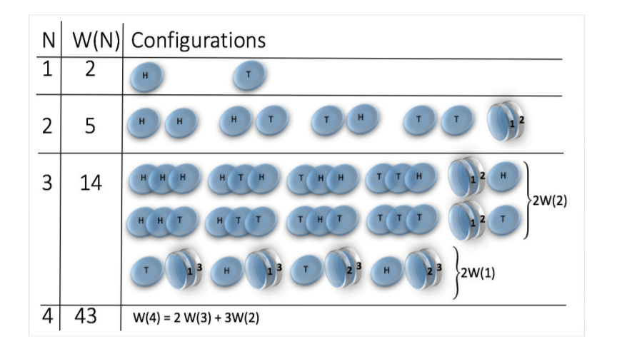
\(W(N) \sim N^N\)

(non-magnetic coins \(W(N) = 2^N\))

H. J. Jensen et al 2018 J. Phys. A: Math. Theor. 51 375002

Boltzmann's entropy

\(S = k_B \log W\)

Multiplicity of structure-forming  systems

Boltzmann entropy formula: \(S(n_i) = k_B \log W(n_i)\) 

where \(W\) is multiplicity

(number of microstates corresponding to a mesostate \(n_i\))

Microstate: state of each particle (if more particles are bound to a molecule, then state of each molecule)

Mesostate: how many particles and/or molecules are in given state

Example: magnetic coin model: 3 coins, magnetic

          microstates                        mesostate                 multiplicity

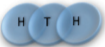
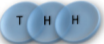
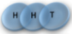
2 x           1x

1 x          1x

3

3

How to calculate a multiplicity?

1. Consider a mesostate
2. Make all permutations of particles
3. Some microstates are overrepresented - calculate how many permutations belong to the same microstate

Examples

2 x           1x

1 x          1x

1    1   2   2    3   3

2   3   1   3    1    2

3   2   3   1    2    1

1    1   2   2    3   3

2   3   1   3    1    2

3   2   3   1    2    1

= (1,2,3) , (2,1,3)

= (1,3,2) , (3,1,2)

= (2,3,1) , (3,2,1)

= (1,2,3) , (1,3,2)

= (2,1,3) , (2,3,1)

= (3,1,2) , (3,2,1)

General formula for multiplicity

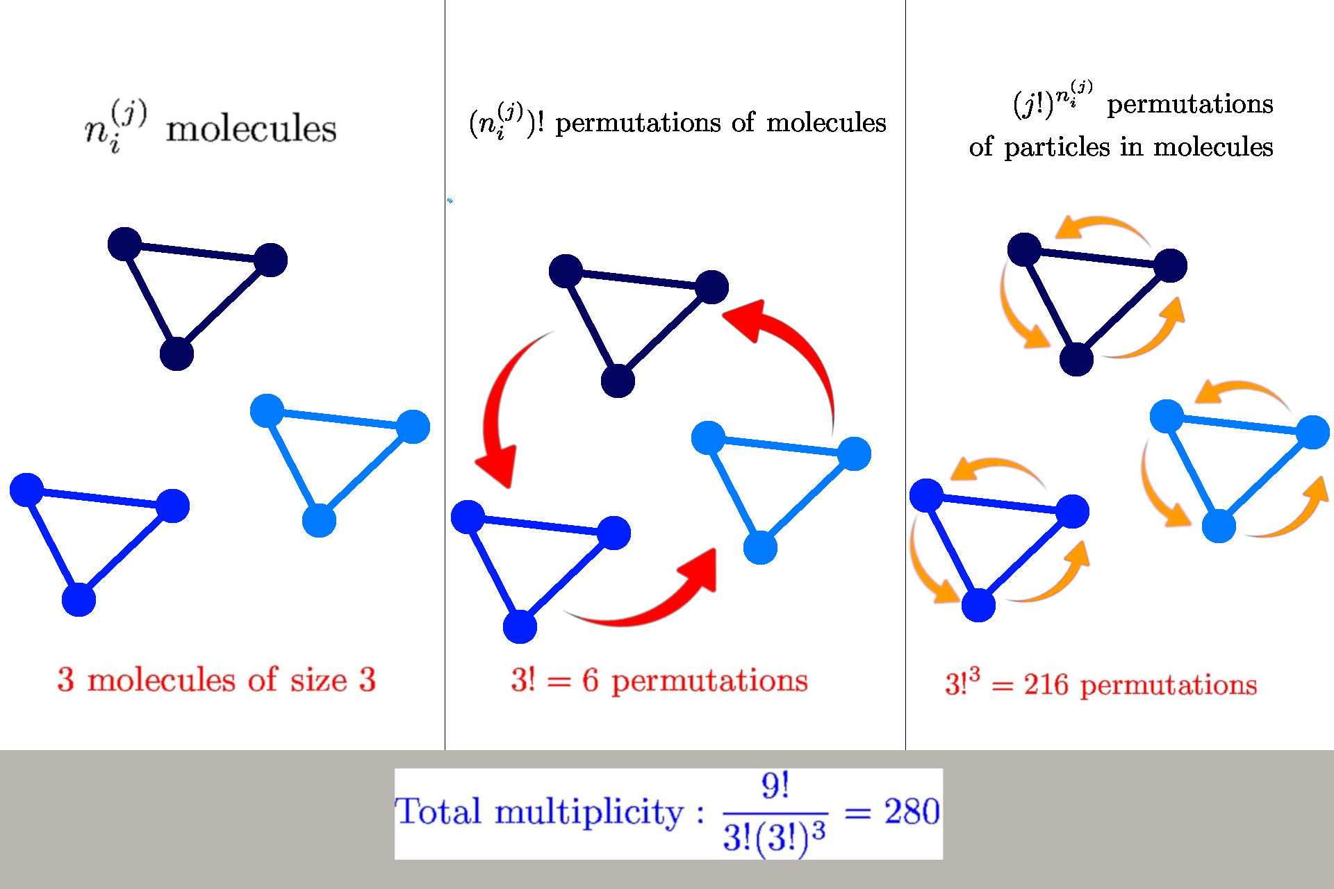
General formula: \(W(n_i^{(j)}) = \frac{n!}{\prod_{ij} n_i^{(j)}!  {\color{red} (j!)^{n_i^{(j)}}}}\)  

we have \(n_i^{(j)}\) molecules of size \(j\) in a state \(s_i^{(j)}\)

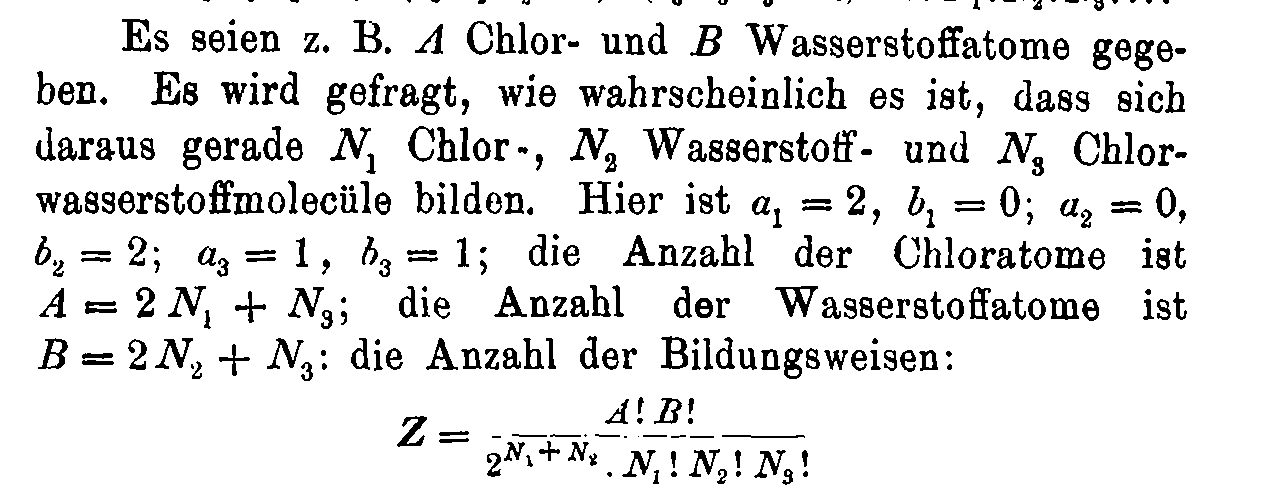
Boltzmann's 1884 paper

Entropy of structure-forming systems

Entropy from Boltzmann's formula using Stirling's approximation

$$ S =  \log W \approx n \log n - \sum_{ij} \left(n_i^{(j)} \log n_i^{(j)} - n_i^{(j)} + {\color{red} n_i^{(j)} \log j!}\right)$$

Introduce "probabilities" \(\wp_i^{(j)} = n_i^{(j)}/n\)

$$\mathcal{S} = S/n = - \sum_{ij} \wp_i^{(j)} (\log \wp_i^{(j)} {\color{red}- 1}) {\color{red}- \sum_{ij} \wp_i^{(j)}\log  \frac{j!}{n^{j-1}}}$$

Normalization: \( \sum_{ij} j \wp_i^{(j)} = 1\)

Finite interaction range: \(b\) boxes, concentration \({\color{blue} c} = n/b\) 

$$\mathcal{S} = S/n = - \sum_{ij} \wp_i^{(j)} (\log \wp_i^{(j)} {\color{red}- 1}) {\color{red}- \sum_{ij} \wp_i^{(j)}\log  \frac{j!}{{\color{blue}c^{j-1}}}}$$

Entropy of structure-forming systems

Axiomatic approaches:

• The entropy fulfills Shannon-Khinchin axioms 1,3,4, but does not fulfill axiom SK 2 (it is not maximized by uniform distribution)
• The entropy fulfills Lieb-Yngvason axioms (it is additive, and it is extensive for \(c=const\) )
• The entropy fulfills Shore-Johnson axioms 1,3,4, but does not fulfill axioms SJ 2 (permutation/coordinate invariance)
• The entropy fulfills Tempesta group-composability axiom but is not symmetric in its arguments
• The scaling exponents according to Hanel-Thurner axioms are              \(c=0,d=1\), the same as for Shannon entropy

\( \Rightarrow\) The entropy satisfies all common axiomatic schemes but it is not symmetric in probabilities

$$\hat{\wp}_i^{(j)} = \frac{c^{j-1}}{j!} \exp(-\alpha j - \beta \epsilon_i^{(j)})$$

MaxEnt distribution

To find the MaxEnt distribution we define Lagrange functional

\(\mathcal{L}(\wp) = S(\wp) - \sum_{ij} j \wp_{i}^{(j)} - \beta \sum_{ij} \epsilon_i^{(j)} \wp_{i}^{(j)} \) 

By maximizing \(\mathcal{L}\) we obtain the MaxEnt distribution

This looks almost like the Boltzmann distribution, but there are a few differences

\(\sum_{ij} j \wp_i^{(j)} = \sum_{ij} \frac{c^{j-1}}{(j-1)!} e^{-{\color{red} \alpha} j - \beta \epsilon_i^{(j)}} = 1\) for \({\color{red} \alpha}\)

Normalization is not obtained by calculating the partition function but by solving

which is a polynomial equation in \(e^{-\alpha}\) of order equal to the maximum size of the molecule

Free energy and cluster-size distribution

Consequently, the free energy can be calculated as

\( F = U - \beta^{-1} S = - \frac{\alpha}{\beta} {\color{red}- \frac{\mathcal{M}}{\beta}}\)

where \(\mathcal{M} = \sum_{ij} \wp_{i}^{(j)}\) is the number of molecules (per particle)

If we focus only on the group-size distribution, we define

\( \wp^{(j)} = \sum_i \wp_i^{(j)}=e^{-j\alpha}  \mathcal{Z}_j\)

where \(\mathcal{Z}_j = \frac{c^{j-1}}{j!}\sum_i e^{-\beta \epsilon_i^{(j)}}\) is the partial partition function

We define the coarse-grained entropy 

\(S_c(\wp) = - \sum_j \wp^{(j)} (\log \wp^{(j)}-1)\)

and partial free energy \(F_j = -\beta^{-1} \ln \mathcal{Z}_j\)

The coarse-grained distribution can be obtained by maximizing  \(L_c(\wp) = S_c(\wp) - \beta \sum_j \wp_j F_j\) 

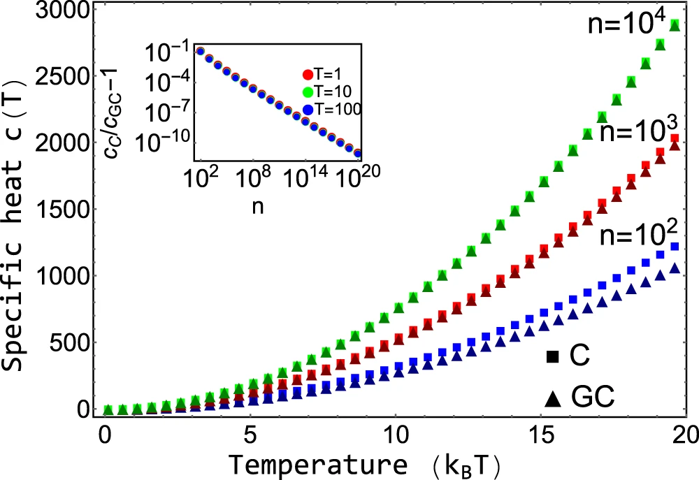
Comparison with grand-canonical ensemble

Stochastic thermodynamics of structure-forming systems

1. Linear Markov (= memoryless) with distribution \(\wp_i(t)\).

Its evolution is described by master equation

$$ \dot{\wp}^{(j)}_i(t) = \sum_{kl} [w_{ik}^{jl} \wp_{k}^{(l)}(t) - w_{ki}^{lj} \wp_i^{(j)}(t) ]$$

\(w_{ij}\) is transition rate. Normalization \(\sum_{ij} j \dot{\wp}_{i}^{(j)}(t) = 0 \)

2. Detailed balance

Assumptions

Stochastic thermodynamics of structure-forming systems

Results

1. Second law of thermodynamics for non-equilibrium systems

2. Detailed fluctuation theorem for structure-forming systems

$$\frac{P(\Delta \sigma)}{\tilde{P}(-\Delta \sigma)} = e^{\Delta \sigma}$$

where  \(\Delta \sigma = \Delta s_i +  {\color{red} \log j_0 - \log j_f}\)

\(\Delta s_i\) is the trajectory entropy production

Applications

 Self-assembly of Janus particles

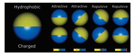
Kern-Frenkel model

Pair-wise potential: \(U^{KF}(r_{ij},n_i,n_j) = u(r_{ij}) \Omega(r_{ij},n_i,n_j) \)

Square-well interaction with hard sphere: 

$$ u(r_{ij}) = \left\{ \begin{array}{rl} \infty, & r_{ij} \leq \sigma \\  - \epsilon, & \sigma < r_{ij} < \sigma + \Delta \\ 0, & r_{ij} > \sigma + \Delta. \end{array} \right.$$

\(\Omega\) decribes orientation of particles:

Particle coverage \(\chi = \sin^2(\theta/2) = \frac{1-\cos{\theta}}{2}\)

Polymers: \(\chi = 0.3\)

Janus particles: \(\chi = 0.5\)

Crystalic structures: \(\chi = 0.6\) (stable lamellar crystals)

$$\Omega(r_{ij},n_i,n_j) = \left\{\begin{array}{rl} -1 & \mathrm{if} \  r_{ij} \cdot n_i > \cos(\theta) \ \mathrm{and} \ r_{ij} \cdot n_j > \cos(\theta)\\ 0 & \mathrm{otherwise} \end{array}  \right.$$

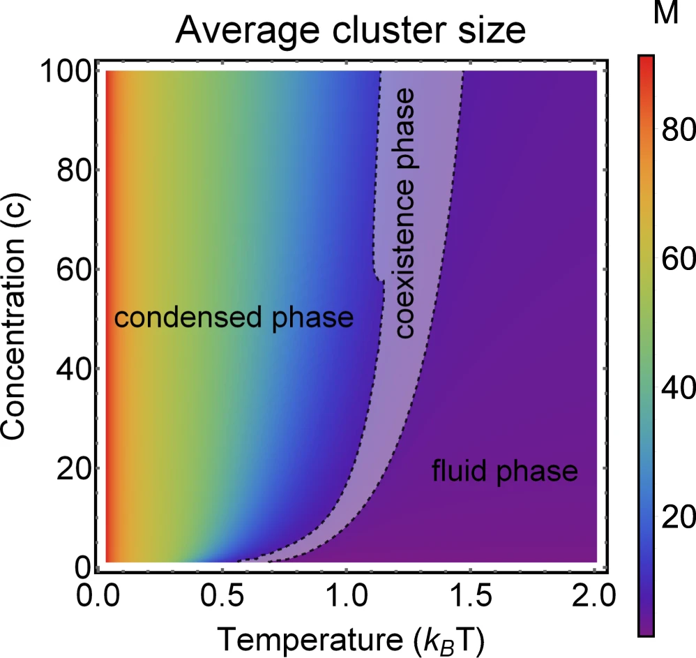
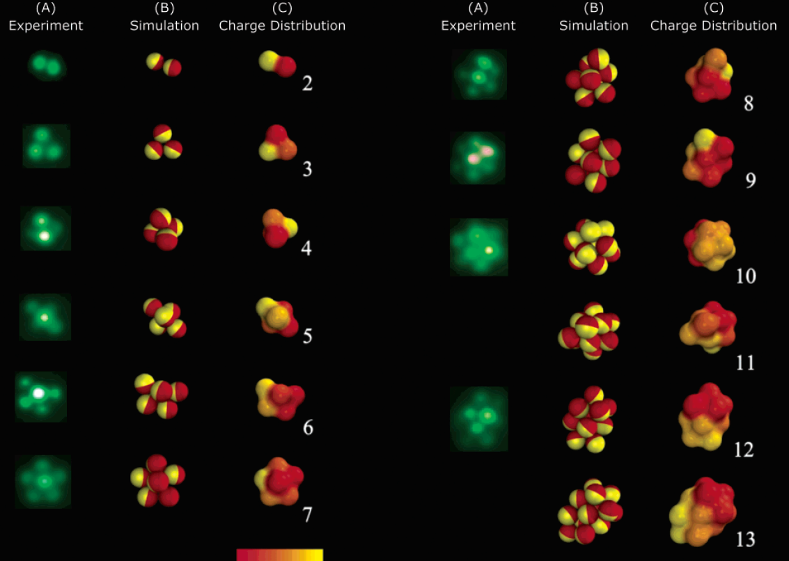
Phase diagram of Janus particles for average cluster size \(M\)

The phase diagram is in agreement with the known theory of self-assembly

Group formation in opinion dynamics model

Driving forces in opinion dynamics

• Many opinion dynamics systems follow two basic concepts:

1. Homophily - people tend to be friends with peers with similar opinions
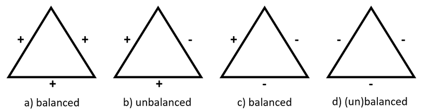
2.  Social balance - a friend of my friend is my friend, enemy of my friend is my enemy

These two concepts can be related through the local Hamiltonian approach

• We introduce a local Hamiltonian (=local stress) based on homophily and show how it is related to social balance
• Each individual has \(G\) binary opinions, \(s_i \in \{-1,1\}^G\)
• If two connected individuals have more common opinions than different opinions, they become friends and vice versa \(J_{ij} = sign(s_i \cdot s_j)\)
• Both homophily and social balance can be incorporated by taking the following social Hamiltonian  $$H(s_i) = -\alpha \sum_{i,j:\mathrm{friends}  } s_i s_j + (1-\alpha) \sum_{i,j: \mathrm{enemies} } s_i s_j$$

Local Hamiltonian approach

Group formation based on homophily

Hamiltonian of a group \(\mathcal{G}\)

\(H(\mathbf{s}_{i_1},\dots,\mathbf{s}_{i_k}) =  \underbrace{- \phi \, \frac{J}{2} \sum_{ij \in \mathcal{G}} A_{ij} \mathbf{s}_i \cdot \mathbf{s}_j}_{\textcolor{red}{intra-group \ social \ stress}}+ \underbrace{(1-\phi) \frac{J}{2} \sum_{i \in \mathcal{G}, j \notin \mathcal{G}} A_{ij} \mathbf{s}_{i} \cdot \mathbf{s}_j}_{\textcolor{aqua}{inter-group \ social \ stress}} \\ \qquad \qquad \qquad \qquad - \underbrace{h \sum_{i \in \mathcal{G}} \mathbf{s}_i \cdot \mathbf{w}}_{external \ field}\)

Group formation based on opinion= self-assembly of spin glass

Group 1

Group 2

Results for zero inter-group degree

Theory

MC simulation

Application online multiplayer game PARDUS

Phase transitions in structure-forming systems

Ising model with molecule formation

Multiplicity on a network

• We derive the multiplicity of a state \(\{n_\uparrow,n_\downarrow,n_\|\}\) 
• The normalization is \(n_\uparrow+n_\downarrow+ 2 n_\| = n\)
• It can be derived as \(W(n_\uparrow,n_\downarrow,n_\|) = \Omega(n_\uparrow,n_\downarrow,n_\|) M(n_\|) \)
• Here, \(\Omega(n_\uparrow,n_\downarrow,n_\|) = \binom{n}{n_\uparrow \ n_\downarrow \ 2 n_\|}\) is the multinomial factor representing the number of divisions of \(n\) particles into the states of the system
• \(M(n_\|)\) represents the number of ways that \(2 n_\|\) particles can form \(n_\|\) molecules
• In fully-connected network, we know it is equal to $$M(n_\|) =  \frac{(2 n_\|)!}{(n_\|)! 2^{n_\|}}$$

Multiplicity on random network

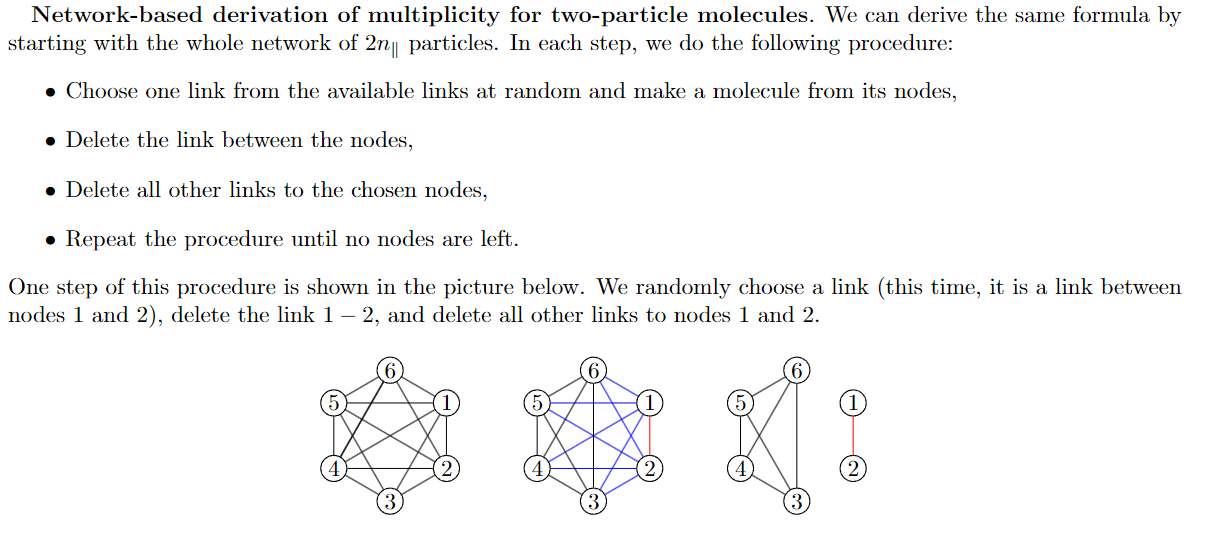
By using the procedure above, we can show that$$M(n_\|) = \frac{1}{(n_\|)!} \prod_{i=0}^{n_\|-1} L(2n_\|-2i)$$

• For each step, we can approximate the number of links by             \(L =  k/(2n)\) where \(k\) is the average degree
• By using this approximation, we end with

$$M(n_\|) =  \frac{(2n_\|)!}{n_\|!} \left(\frac{k}{2(n-1)}\right)^{n_\|} $$

Entropy of Ising model with molecules

• Entropy can be expressed from \(S \equiv \log W = \log (\Omega M) \)  
• It leads to $$S(\wp_\uparrow,\wp_\downarrow,\wp_\|) = - \wp_\uparrow (\log \wp_\uparrow - 1) - \wp_\downarrow (\log \wp_\downarrow - 1)$$  $$- \wp_\| (\log \wp_\| - 1)- \wp_\| \log \left(\frac{2(n-1)}{k n}\right) $$ 
• By solving the self-consistency equation, we observe the transition between second-order and first-order transtion

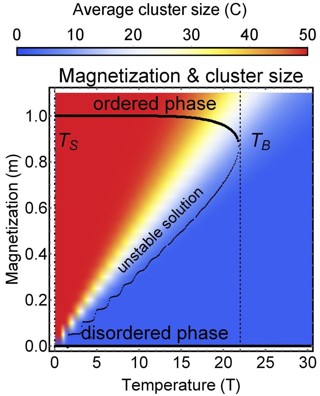
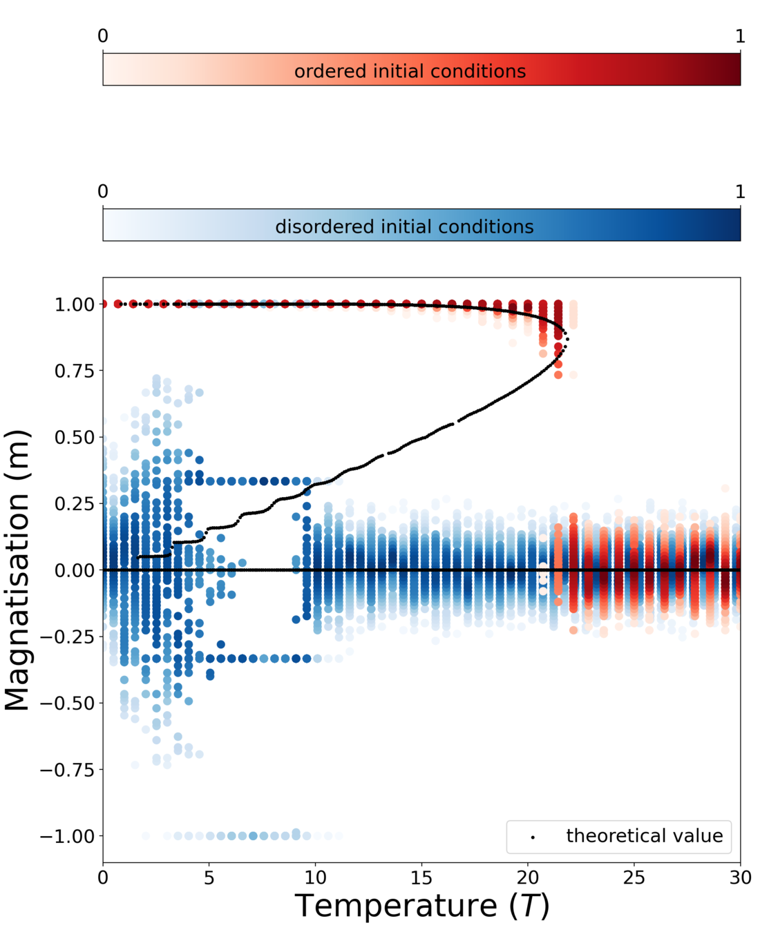
Phase diagram

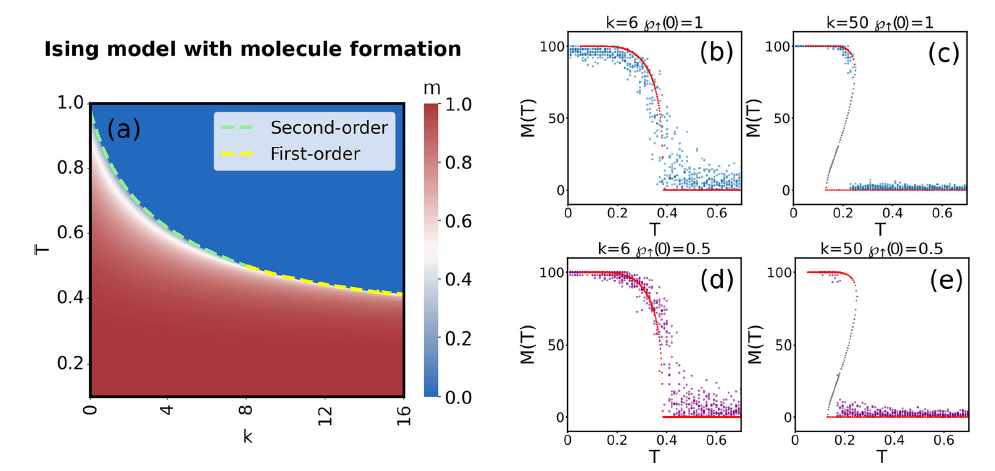
$$m =   \frac{2 \left(- \cosh( \beta J m) + \sqrt{  \cosh^2(\beta J m) + k}\right)}{k} \sinh (\beta J m )$$

Microscopic origin of abrupt phase transition

csh.ac.at

Conclusions

• Many real-world systems form structures
• Their thermodynamics can be described in terms of the canonical ensemble
• We obtain entropy for structure-forming systems
• The results have applications in soft matter, sociophysics and critical phase transitions

csh.ac.at

In collaboration with:

Stefan Thurner

Rudolf Hanel

Tuan Pham Minh

Simon Lindner

Shlomo Havlin

Slides available at: slides.com/jankorbel

Personal web: jankorbel.eu

Thank you for your attention