Drivers of Social Polarization: Insights from Social Connectivity and Campaign Influence

Jan Korbel
web: jankorbel.eu
slides: slides.com/jankorbel


Part one:
Paper flow
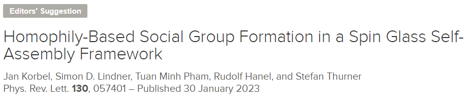
1.
2.
3.
1. Thermodynamics of
structure-forming systems
Entropy for systems with structures
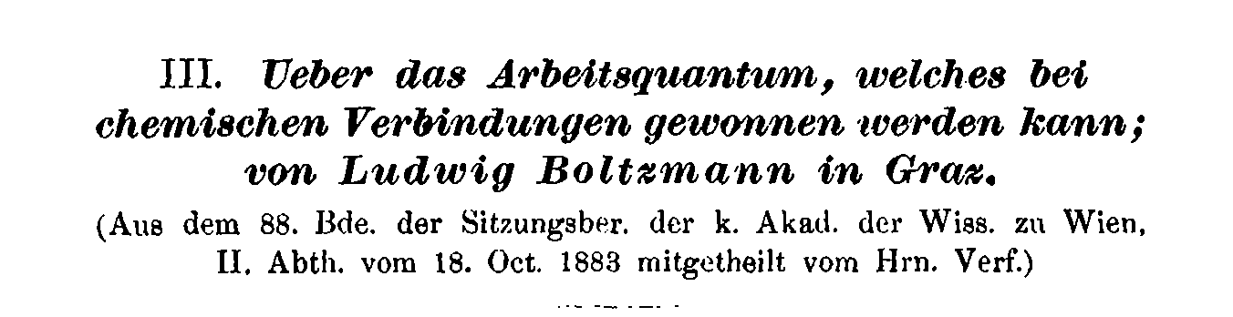
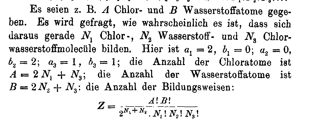
\(W(n_i^{(j)}) = \frac{n!}{\prod_{ij} n_i^{(j)}! \textcolor{red}{(j!)^{n_i^{(j)}}}}\)
$$\mathcal{S} = - \sum_{ij} \wp_i^{(j)} (\log \wp_i^{(j)} {\color{red}- 1}) {\color{red}- \sum_{ij} \wp_i^{(j)}\log \frac{j!}{n^{j-1}}}$$

\( S = k \cdot \log W\)

\( \wp_i^{(j)} = n_i^{(j)}/n\)
When we want to calculate the MaxEnt distribution, we maximize the entropy w.r.t. to
- normalization \(\sum_{ij} j \wp_{i}^{(j)}=1\)
- average energy \(\sum_{ij} \wp_{i}^{(j)} \epsilon_{i}^{(j)} = E\)
Equilibrium distribution:
$$\hat{\wp}_i^{(j)} = \frac{n^{j-1}}{j!} \exp(-\alpha j - \beta \epsilon_i^{(j)})$$
Normalization:
\(\sum_{ij} j \wp_i^{(j)} = \sum_{ij} \frac{n^{j-1}}{(j-1)!} e^{-{\color{red} \alpha} j - \beta \epsilon_i^{(j)}} = 1\) for \({\color{red} \alpha}\)
Free energy:
\( F = U - \beta^{-1} S = - \frac{\alpha}{\beta} {\color{red}- \frac{\mathcal{M}}{\beta}}\)
where \(\mathcal{M} = \sum_{ij} \wp_{i}^{(j)}\) is the number of molecules
MaxEnt distribution and free energy
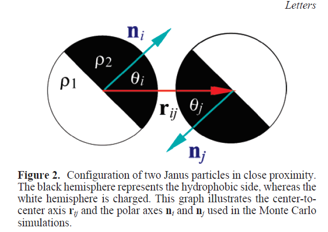
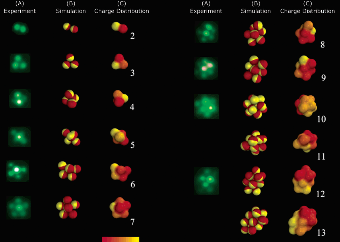
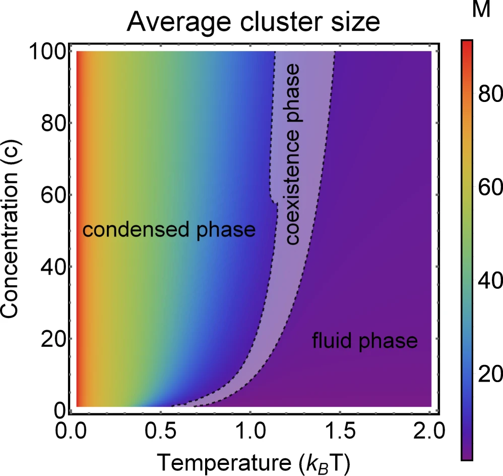
Applications to self-assembly
2. Spin-glass based opinion dynamics
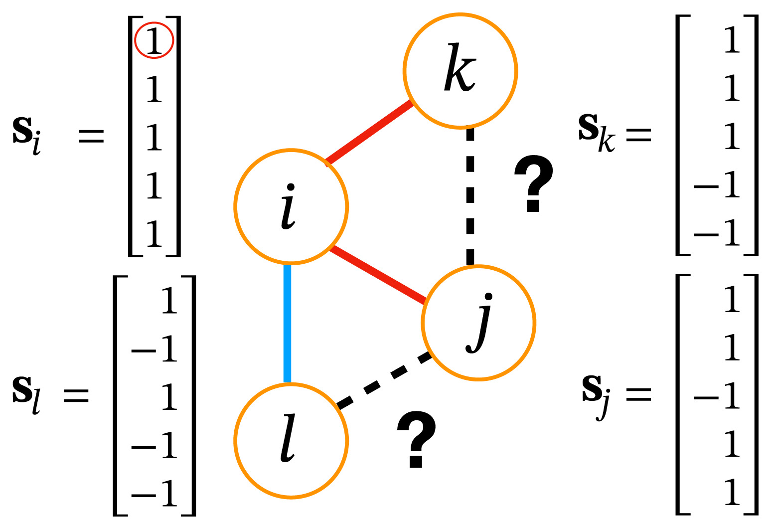
- Many opinion dynamics systems follow two basic concepts:
1. Homophily - people tend to be friends with peers with similar opinions ("birds of a feather flock together")

2.Social balance - people tend to follow Heider balance relation
("a friend of my friend is my friend, enemy of my friend is my enemy")
2. Spin-glass based opinion dynamics

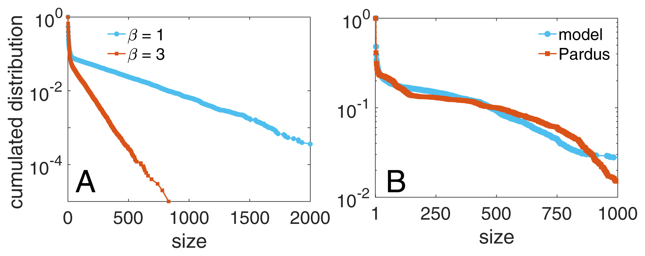
Group size distribution
Social balance can emerge from homophily
3. Social group formation in the spin-glass self-assembly framework
Hamiltonian of a group \(\mathcal{G}\)
\(H(\mathbf{s}_{i_1},\dots,\mathbf{s}_{i_k}) = \textcolor{red}{\underbrace{- \phi \, \frac{J}{2} \sum_{ij \in \mathcal{G}} A_{ij} \mathbf{s}_i \cdot \mathbf{s}_j}_{intra-group \ social \ stress}} \textcolor{blue}{ + \underbrace{(1-\phi) \frac{J}{2} \sum_{i \in \mathcal{G}, j \notin \mathcal{G}} A_{ij} \mathbf{s}_{i} \cdot \mathbf{s}_j}_{inter-group \ social \ stress}} \\ \qquad \qquad \qquad \qquad - \underbrace{h \sum_{i \in \mathcal{G}} \mathbf{s}_i \cdot \mathbf{w}}_{external \ field}\)
Group formation based on opinion= self-assembly of spin glass
Group 1
Group 2
friends
enemies
Approximations used in the model
1. Configuration model
- We do not know the full network, just a degree distribution. \(\Rightarrow\) The probability of observing a link between \(i\) and \(j\) is proportional to the degree of both nodes
2. Mean-field approximation
- We use the mean-field approximation of the Hamiltonian.
These two approximations lead to the set of self-consistency equations:
$$m^{(k)} = k \sum_{q^{(k)} q^{(k,l)}} P(q^{(k)}) P(q^{(k,l)}) \tanh(\beta H^{(k)}(m^{(l)},q^{(k)},q^{(k,l)})) $$
where \(q^{(k)}\) is the intra-group degree, \(q^{(k,l)}\) is the inter-group degree and \(P\) is the degree distribution
Results for zero inter-group degree
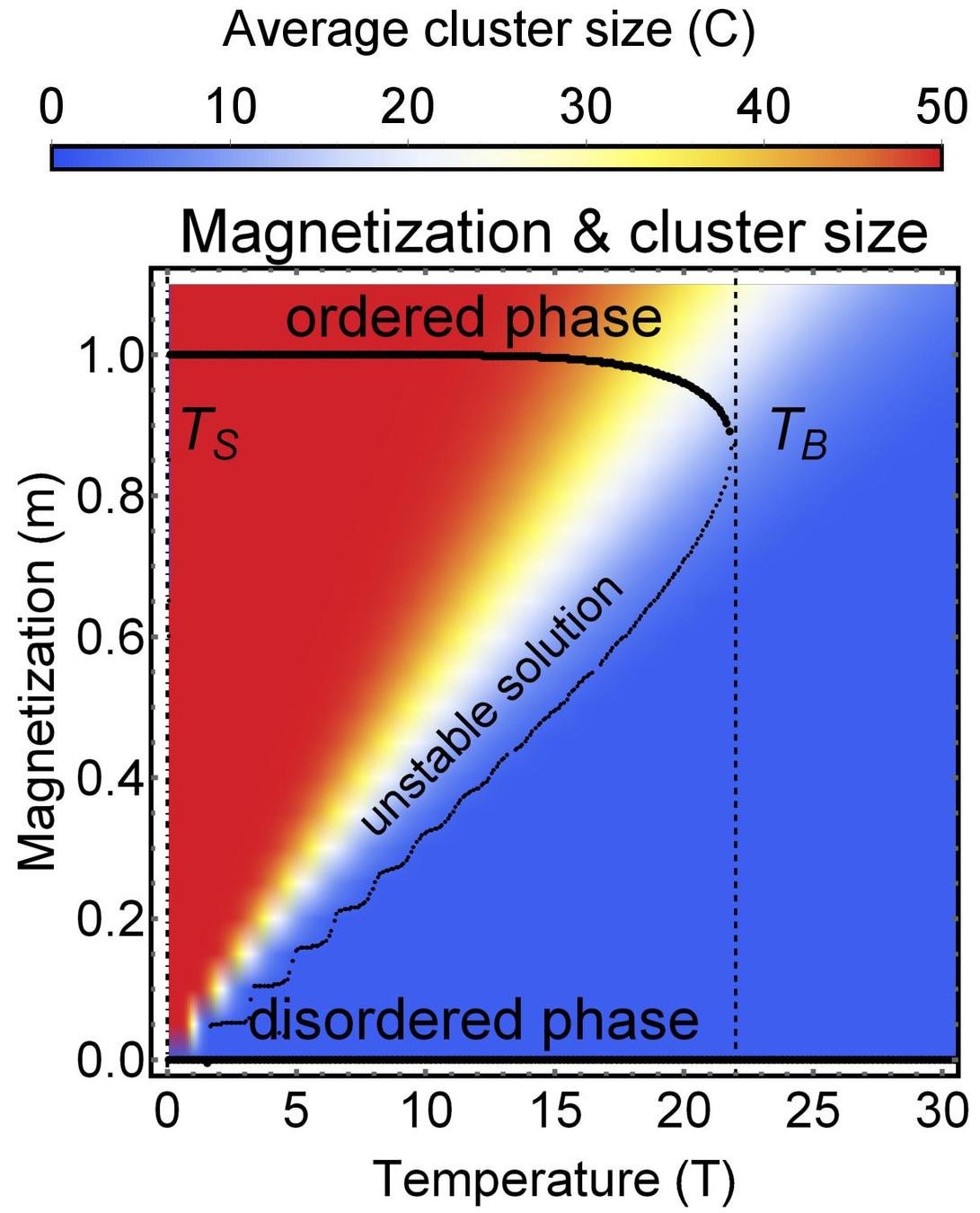
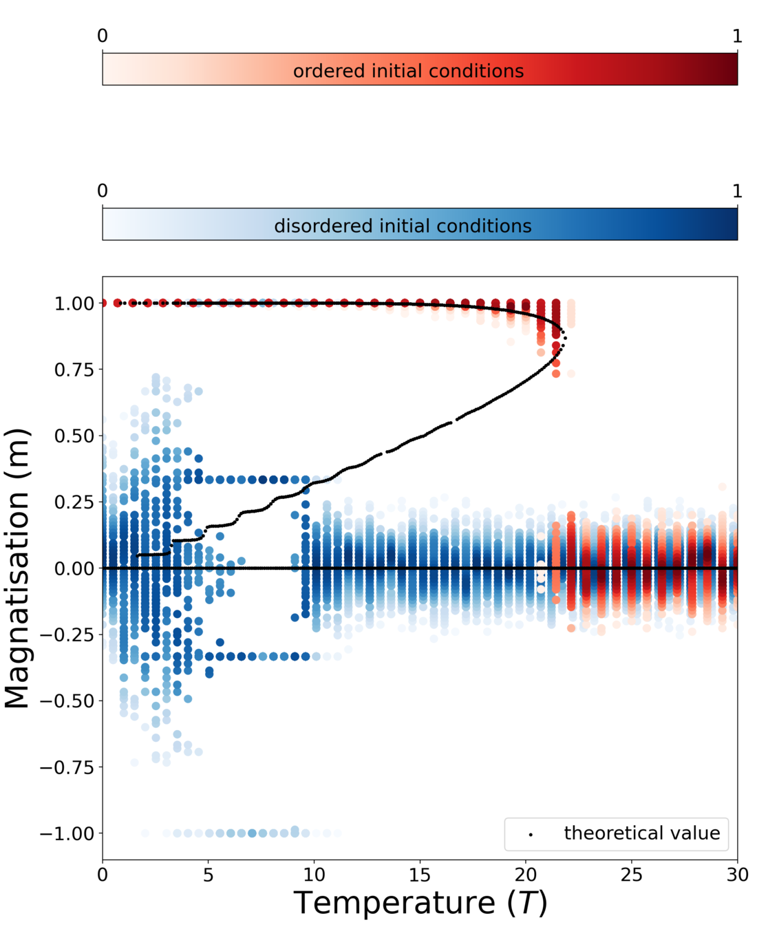
Theory
MC simulation

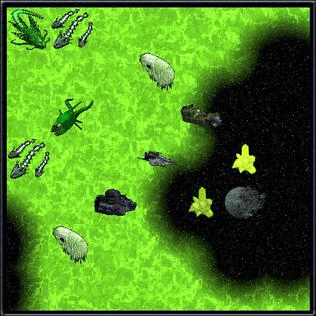
Application online multiplayer game PARDUS
Part two:

Motivation
Recent elections show increasing political polarization.
However, it is unclear how campaign spending interacts with social influence among voters.
Key question:
How does campaign spending influence this polarization?
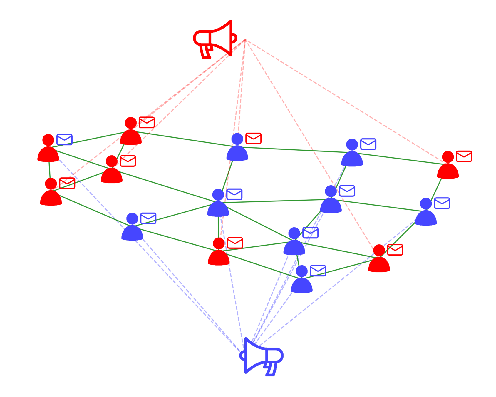
We use a simple physics-inspired model combining two key factors: voter homophily and campaign intensity.
Illustration of the model
Ising model with random bimodal field
- We model the individual opinion as a binary spin $$s_i \in \{-1,+1\}$$
- The homophily is given by the standard Ising model $$ - J \sum_{ij} A_{ij} s_i s_j \quad \textrm{where} \ A_{ij} \textrm{\ is \ adj. \ matrix} $$
- The external campaign is given by the random external field $$- \sum_i h_i s_i \quad \textrm{where} \ h_i \in \{+h^+,-h^-\}$$
- Here \(h^+\) denotes the intensity of the campaign to promote opinion \(s = +1\) and \(h^-\) is the intensity of the campaign to promote opinion \(s = -1\)
Mean-field approximation
- The Hamiltonian describes a Random-Field Ising model $$H(s) = - J\sum_{ij} A_{ij} s_i s_j - \sum_i h_i s_i$$ with a bimodal (and binary) field
- By using mean-field approximation and configuration model approximation we obtain $$H^{MF}(s) = - \sum_i (\tilde{J} m + h_i) \sigma_i$$ where \(\tilde{J} = J/\langle k \rangle\) and \(h_i\) is a binary random variable with the probability distribution \((p(h^+),p(h^-))\) where \(p \equiv p({h^+})\)
- The random component models affiliation to one or the other campaign
Self-consistency equation
- By averaging of the random field, the opinion distribution is $$p(s) = \frac{p e^{- \beta(\tilde{J} m + {h^+}) s) } + (1-p) e^{-\beta (\tilde{J} m - h^-)s}}{Z}$$
- The average magnetization can be determined as $$m = \langle s \rangle = p \langle s \rangle_{h=h^+}+ (1-p) \langle s \rangle_{h=h^-}$$ from which we get the self-consistency equation
$$m= p \tanh(\beta(\tilde{J} m + h^+)) + (1-p) \tanh(\beta \tilde{J} m - h^-)$$
Critical point and phase transition
- For \(T \geq 1\), we observe no phase transition
- For \(T<1\) we observe a phase transition where the transition is observed at critical points$$h_c^+ = T \, \textrm{arctanh}\left(\sqrt{(1-T) \frac{1-p}{p}}\right)$$$$h_c^- = T \, \textrm{arctanh}\left(\sqrt{(1-T) \frac{p}{1-p}}\right)$$
- This is a generalization of the well-known critical curve for symmetric case \( (p=1/2) \)
- Thus, for \(T<1\) the system has a hysteresis region
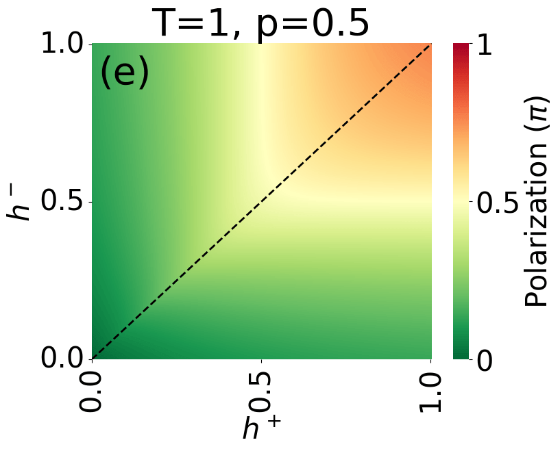
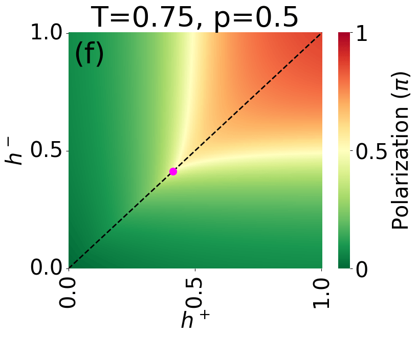
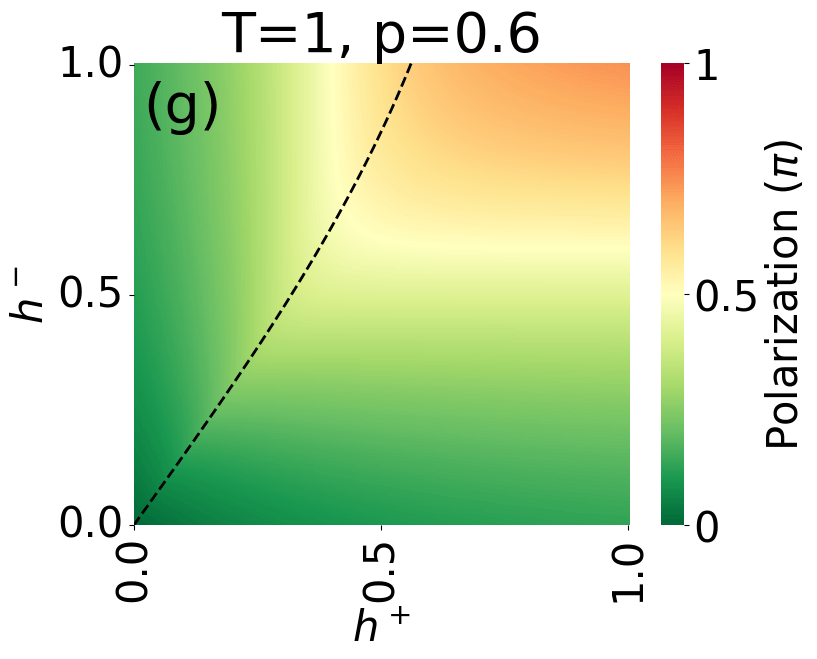
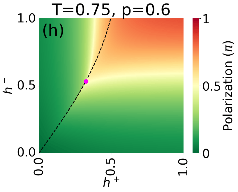
Polarization
- To measure whether the society is in consensus or polarized, we define a quantity
$$\pi = \frac{1}{2} \left( \langle s \rangle_{h=h^+} - \langle s \rangle_{h=h^-} \right)$$
- This quantity, which is called campaign polarization, measures the difference between the opinion of groups affected by the opposite campaigns.
Phase diagrams
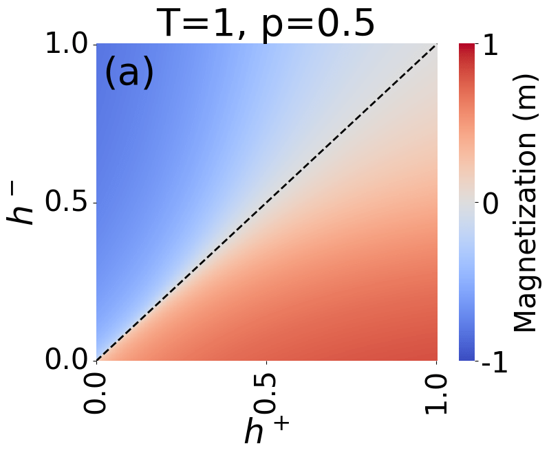
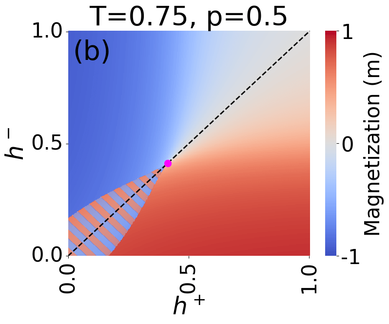
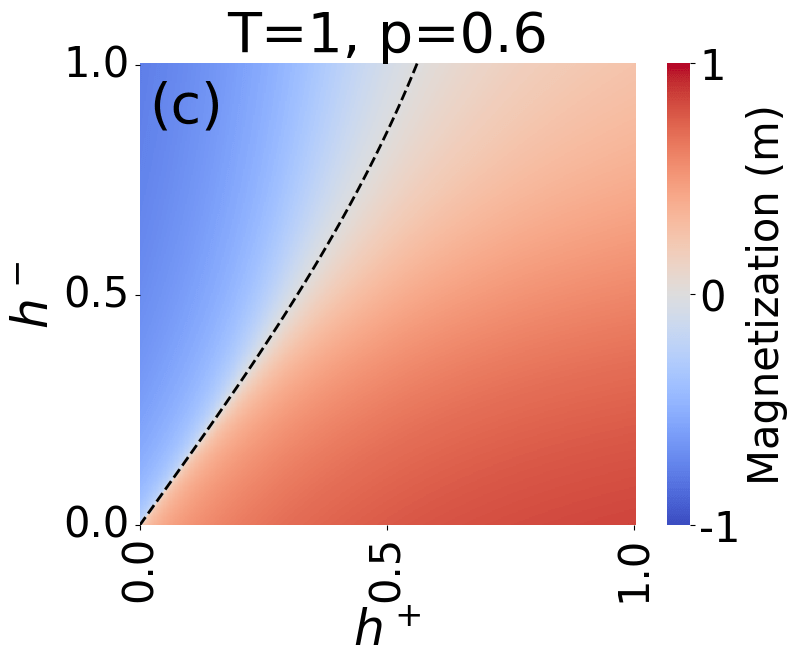
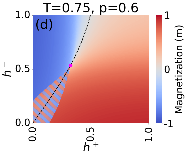
Magnetization
Polarization
Application to US House elections 1980-2020
- We apply our model to the US House elections
- We include only bipartisan races (all races with more than 2 candidates with non-negligible outcome are excluded)
- Altogether, we analyze 6357 races
- We use our model as a winner classifier
- If m>0, the Republican wins
- If m<0 , the Democrat wins
- The hysteresis region is interpreted as incumbency region (i.e., incumbent wins even if they spend less)
- We use the hysteresis region to calibrate the model parameters \(T\) and \(h_c\)
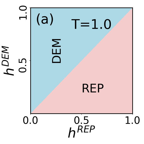
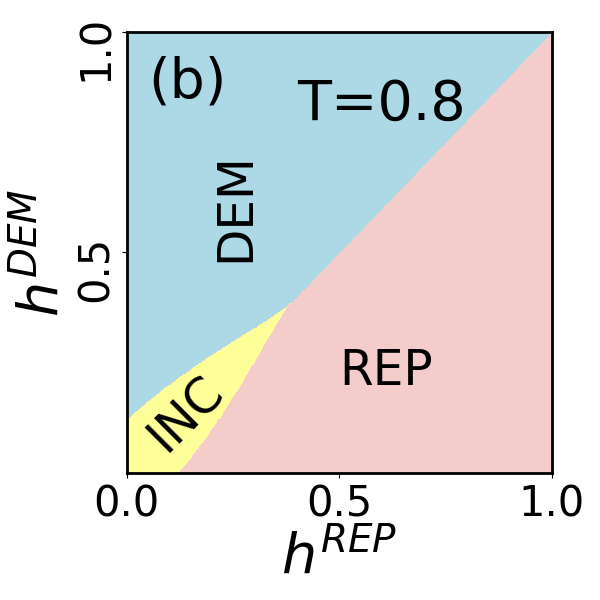
Classifiers
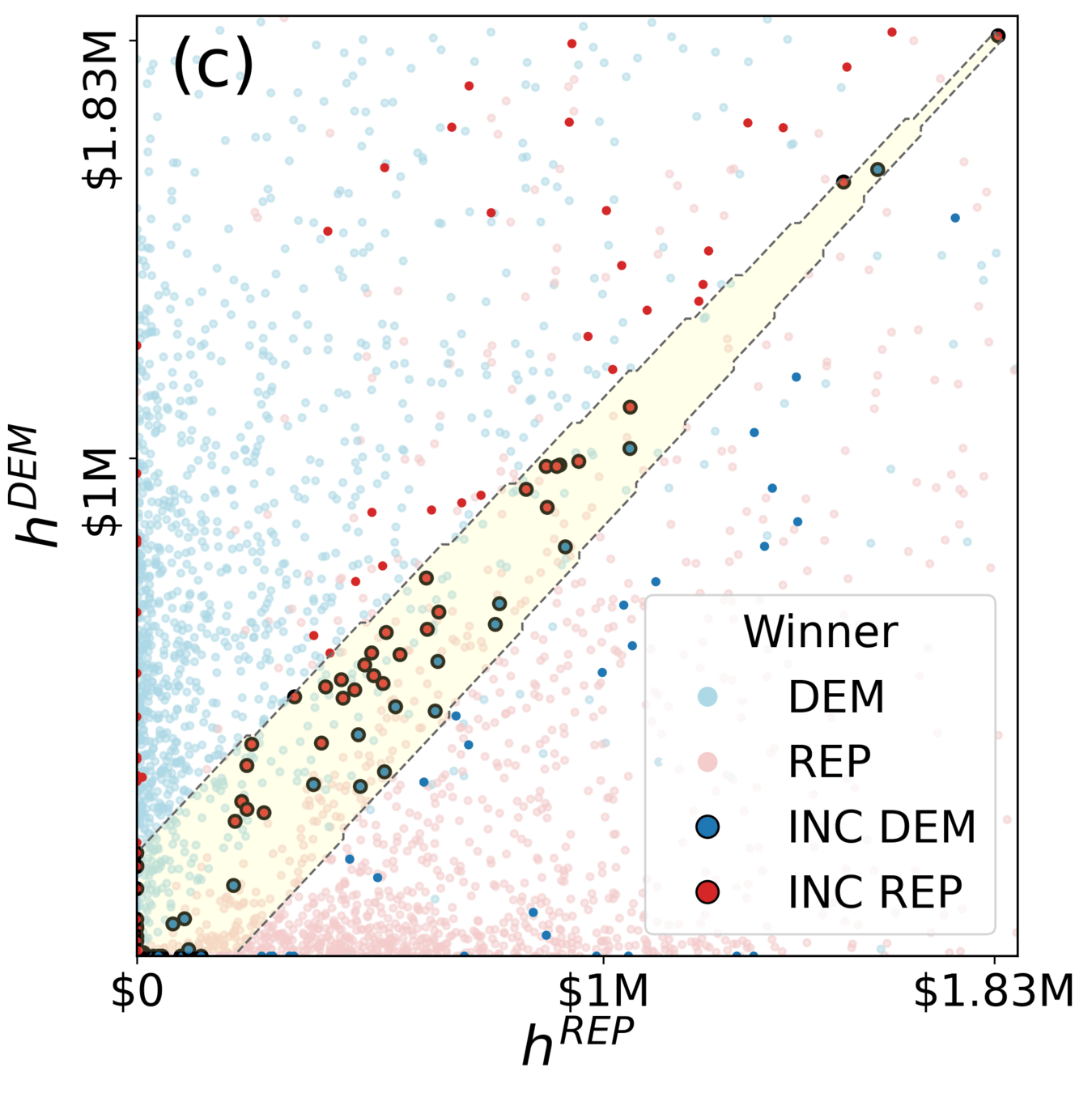
incumbency region
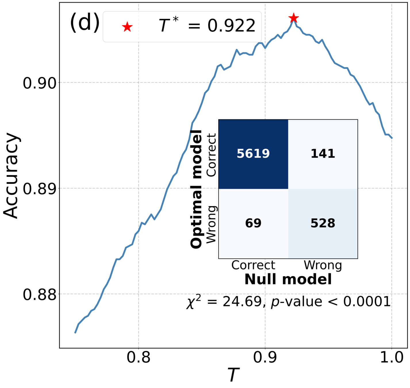
optimal temperature
Application to US House elections 1980-2020
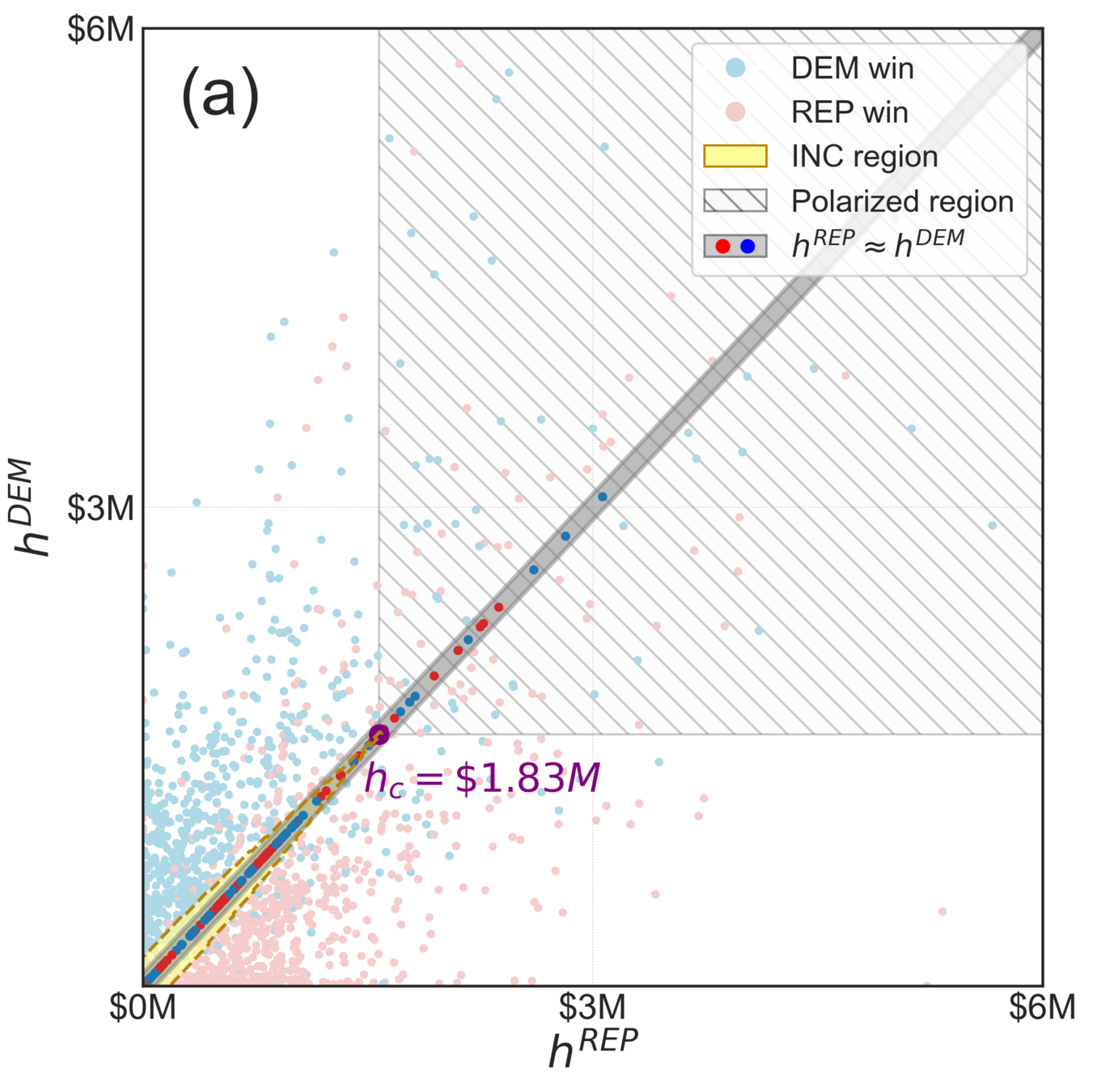
full region
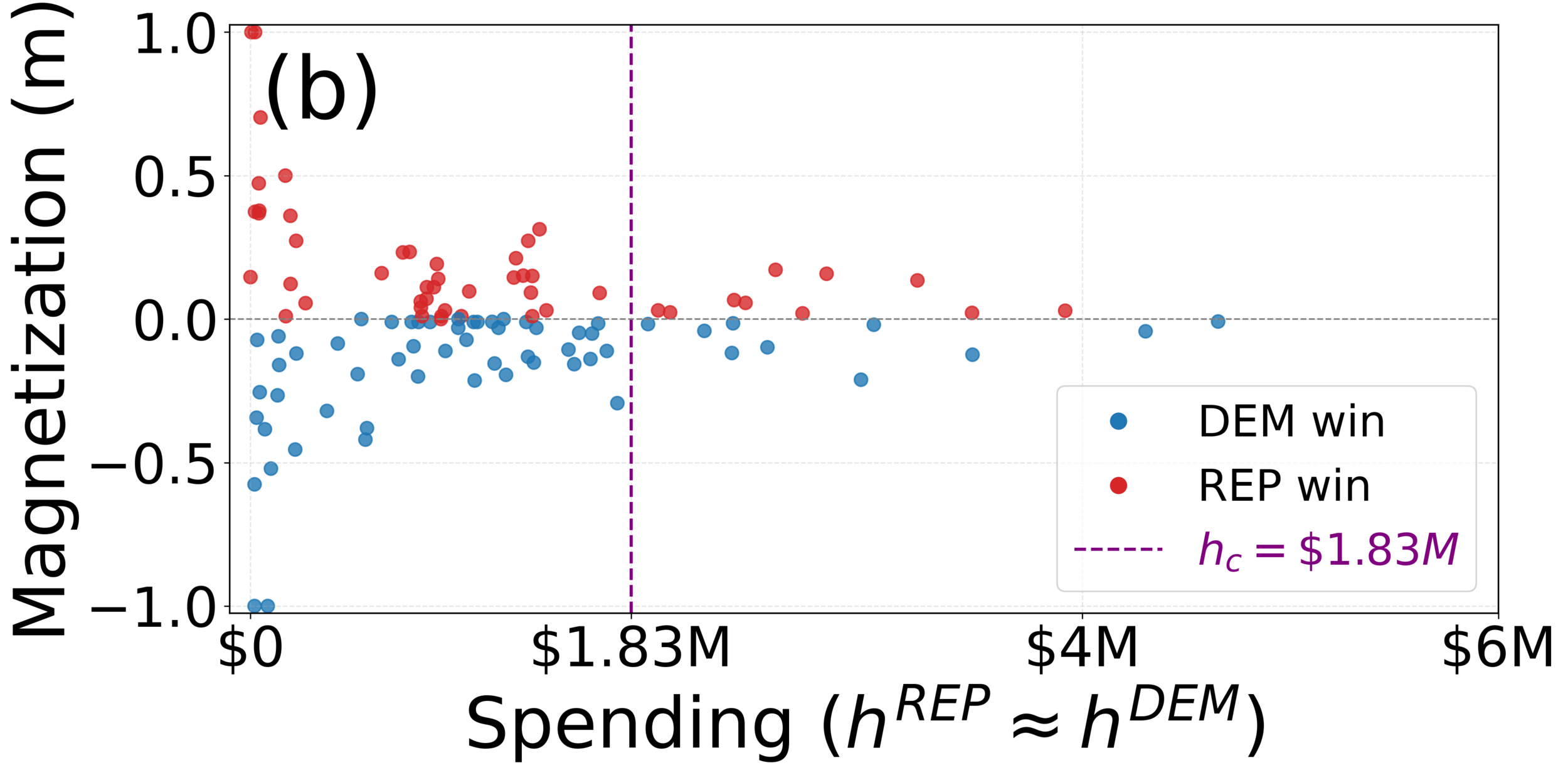
results for close races
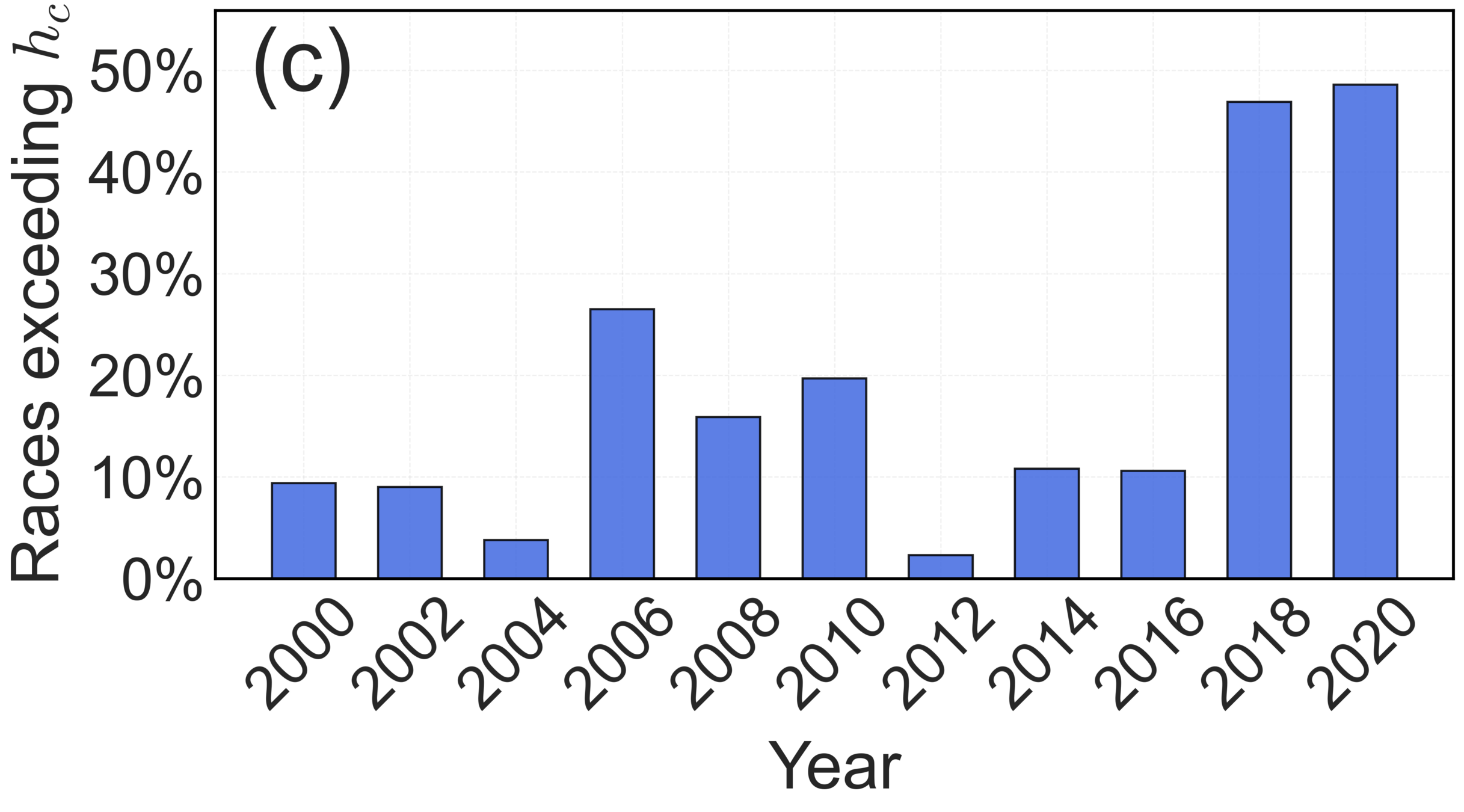
spending above \(h_c\)
Application to US House elections 1980-2020
Acknowledments
Funders
qr code
csh.ac.at
Drivers of Social Polarization: Insights from Social Connectivity and Campaign influence
By Jan Korbel