


Juan Carlos Ponce Campuzano
Mathematics Educator
Juan Carlos Ponce Campuzano
School of Environment and Science
A mysterious curve
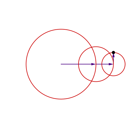
A circle moving on another circle.
A circle moving on another circle, on another circle.
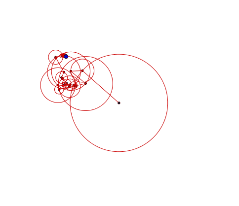
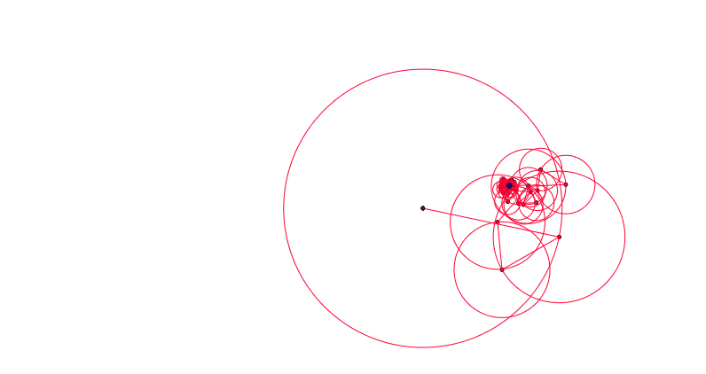
A circle moving on another circle, on another circle, on another circle...
How can we represent them mathematically?
A parametric function!
🔍
Code:
ABEV FXP8
🔍
Work only with
Code:
ABEV FXP8
Both represent
the same thing!
\(\sin x\)
\(\sin x\) and \(\cos x\)
👉
Complete last task!
6
-14
6
-14
Why there is rotational symmetry?
6
-14
Is this symmetry related to these numbers?
A parametric function with sin and cos functions
In general we have:
This new symbol \(\phi_k\) indicates how much the disk \(k\) is initially rotated at time \(t = 0\), and we called a phase offset.
If we do not specify a phase offset, we can only describe epicycles where the circles start aligned.
\(\phi_k\) is called a phase offset
Using properties of complex numbers:
\(i\cdot i = -1\)
Discrete Fourier Transform
\(\Bigg\{\Bigg.\)
Discrete Fourier Transform
👈 DFT
The inverse of the DFT
👈
(DFT)
They are very similar to this:
\(\Bigg\{\Bigg.\)
Discrete Fourier Transform
(DFT)
They are very similar to this:
\(\Bigg\{\Bigg.\)
Discrete Fourier Transform
(DFT)
Discrete Fourier Transform
(DFT)
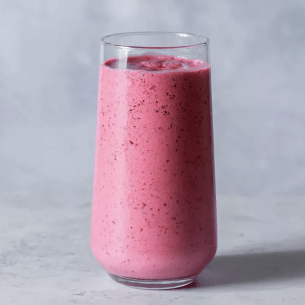
A nice methaphor 😃
What does the Discrete Fourier Transform do?
Given a smoothie, it finds the recipe.
A nice methaphor 😃
🍓 🍌🥭🍏
🫐🍍🥝🍫
How does it do that?
A nice methaphor 😃
How does it do that?
Run the smoothie through filters to extract each ingredient.
🍓 🍌🥭🍏
🫐🍍🥝🍫
A nice methaphor 😃
🍓 🍌🥭🍏
🫐🍍🥝🍫
Why do we want to do this?
Recipes are easy to analyse, compare, than the smoothie itself.
A nice methaphor 😃
🍓 🍌🥭🍏
🫐🍍🥝🍫
How do we get the smoothie back?
Blend the ingredients.
A nice methaphor 😃
🍓 🍌🥭🍏
🫐🍍🥝🍫
How do we get the smoothie back?
Blend the ingredients.
Applications of the DFT
Modern digital media
Applications of the DFT
Video
Applications of the DFT
Images
Applications of the DFT
Magnetic Resonance Imaging
Applications of the DFT
Sound
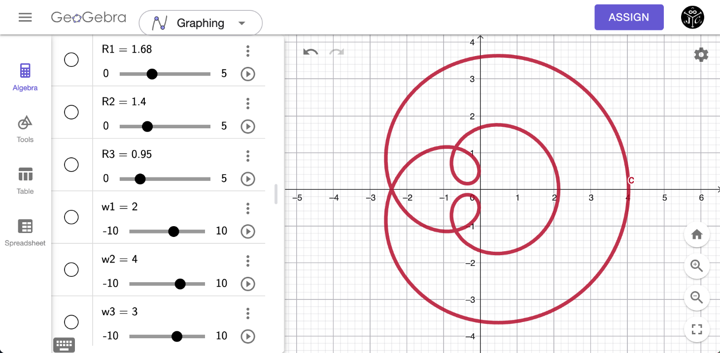
Try it yourself!
R1 = Slider(0, 5, 0.01, 1, 200)
R2 = Slider(0, 5, 0.01, 1, 200)
R3 = Slider(0, 5, 0.01, 1, 200)
w1 = Slider(-10, 10, 1, 1, 200)
w2 = Slider(-10, 10, 1, 1, 200)
w3 = Slider(-10, 10, 1, 1, 200)
fx(x) = R1 * cos(w1 * x) + R2 * cos(w2 * x) + R3 * cos(w3 * x)
fy(x) = R1 * sin(w1 * x) + R2 * sin(w2 * x) + R3 * sin(w3 * x)
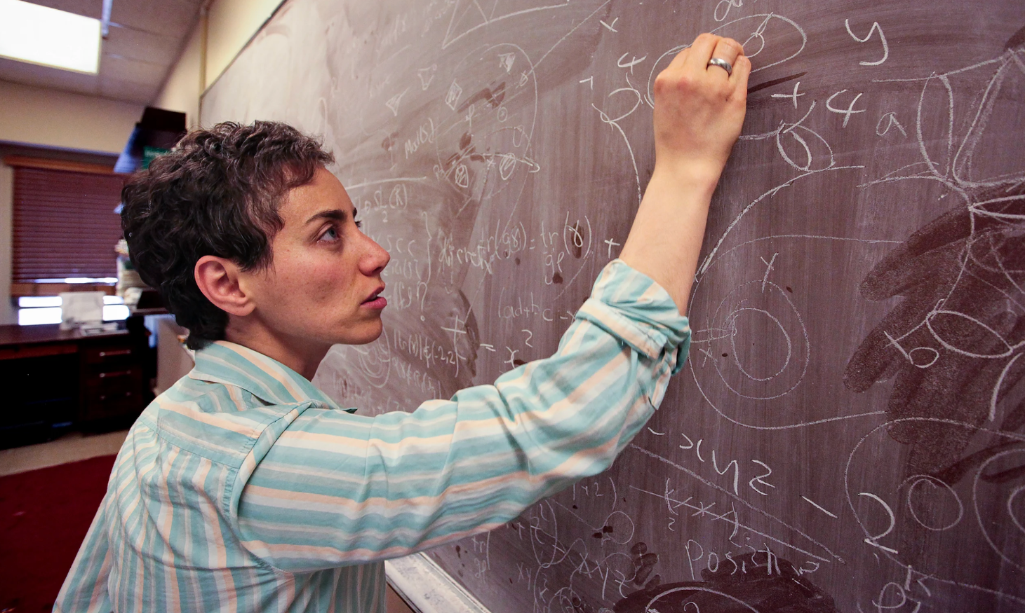
c = Curve(fx(t), fy(t), t, 0, 2pi)The beauty of mathematics shows itself to patient followers.
- Maryam Mirzakhani
By Juan Carlos Ponce Campuzano
The mathematical beauty of epicycles


