


Juan Carlos Ponce Campuzano
Mathematics Educator
System of differential equations
Non-linear system of
ordinary differential equations (ODEs)
\(\dfrac{dx}{dt}=x'\)
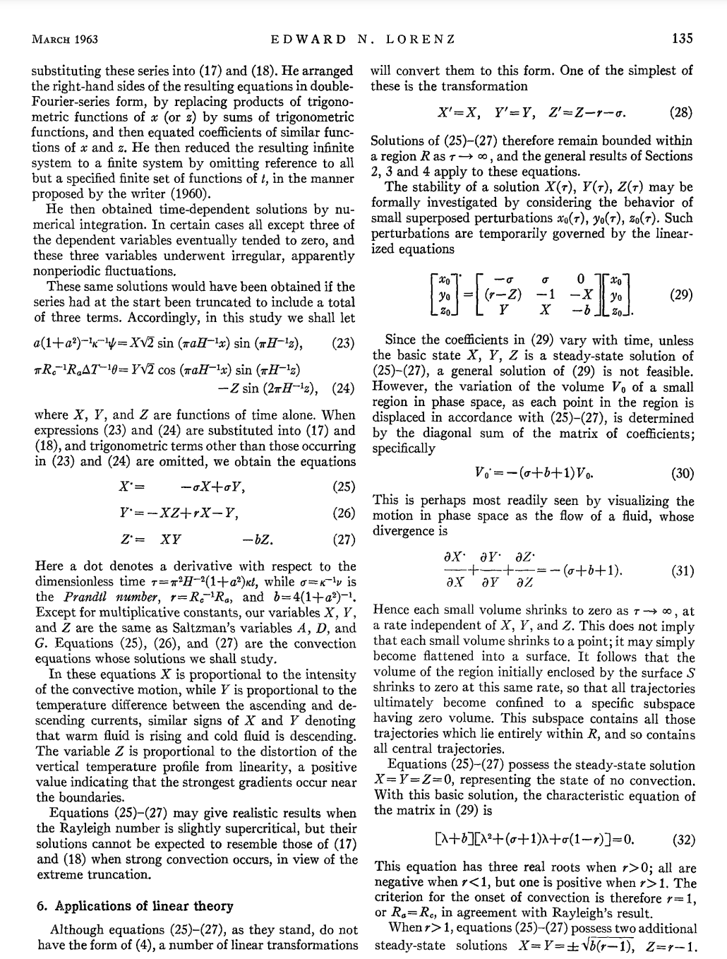
Lorenz E. N. (1963). Deterministic Nonperiodic Flow. Journal of the Atmospheric Sciences. 20(2): 130–141.
It was introduced in the 1960s
by Edward Norton Lorenz
Lorenz E. N. (1963). Deterministic Nonperiodic Flow. Journal of the Atmospheric Sciences. 20(2): 130–141.
as a simplified mathematical model
for the atmospheric convection.
It was introduced in the 1960s
by Edward Norton Lorenz
We are looking for the functions
such that
What does it mean to solve a system?
\((x,y,z)\)
\(x\)
\(y\)
\(z\)
The solution gives you the position
If the system represents the velocity of this particle
time
\(t\)
\((x,y,z)\)
\(x\)
\(y\)
\(z\)
time
\(t\)
The solution gives you the position
at any time \(t\)
In general, solving systems of ODEs is incredibly difficult,
sometimes even impossible!
The good news are that we still can solve them numerically!
In GeoGebra we can use the command
NSolveODE()Here is where computers are quite useful
NSolveODE(
	List of Derivatives,
 	Initial x-coordinate,
 	List of Initial y-coordinates,
 	Final x-coordinate
) NSolveODE()Initial time
\(t_0\)
Initial conditions
\((x_0,y_0,z_0)\) at \(t=t_0\)
Final time
\(t_f\)
\((x_0,y_0,z_0)\)
\(x\)
\(y\)
\(z\)
time
\(t\)
\(t_0\)
\(t_f\)
\(x\)
\(y\)
\(z\)
time
\(t\)
\(t_0\)
\(t_f\)
\((x_f,y_f,z_f)\)
\((x_0,y_0,z_0)\)
d = 10
b = 8/3
p = 28

x'(t,x,y,z) = d * (y - x)
y'(t,x,y,z) = x * (p - z) - y
z'(t,x,y,z) = x * y - b * z

x0 = 1
y0 = 1
z0 = 1

NSolveODE({x', y', z'}, 0, {x0, y0, z0}, 20)

len = Length(numericalIntegral1)

L_1 = Sequence( (y(Point(numericalIntegral1, i)), y(Point(numericalIntegral2, i)), y(Point(numericalIntegral3, i))), i, 0, 1, 1 / len )

f = Polyline(L_1)The algorithm behind this command is based on
Runge-Kutta numeric methods
NSolveODE()NSolveODE(
List of Derivatives,
Initial x-coordinate,
List of Initial y-coordinates,
Final x-coordinate
)By Juan Carlos Ponce Campuzano
Lorenz attractor in GeoGebra: https://youtu.be/8_BLhxjrho0


