Learned Proximal Operators
from denoising to sampling
Jeremias Sulam



A central question in data science
observation
model of the world
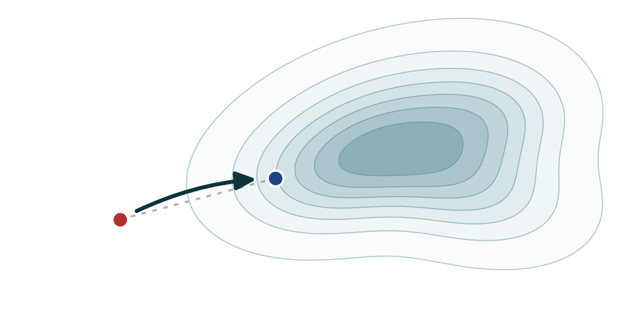
Inverse Problems
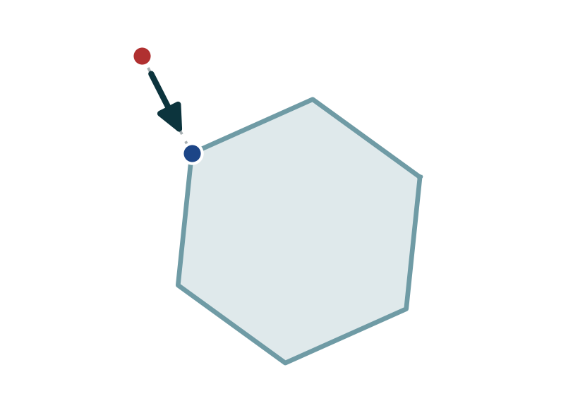
Constrained Optimization
Sampling
Outlier Detection
A central question in data science
Sampling
Outlier Detection
A central question in data science
Inverse Problems
Today: how we learn these operators from data?
Proximal Operators
Constrained Optimization
Proximal Operators
\text{prox}_{\lambda R}(y) ~\triangleq~ \underset{x}{\arg\min} ~ \tfrac12 \|x-y\|_2^2 + \lambda R(x)
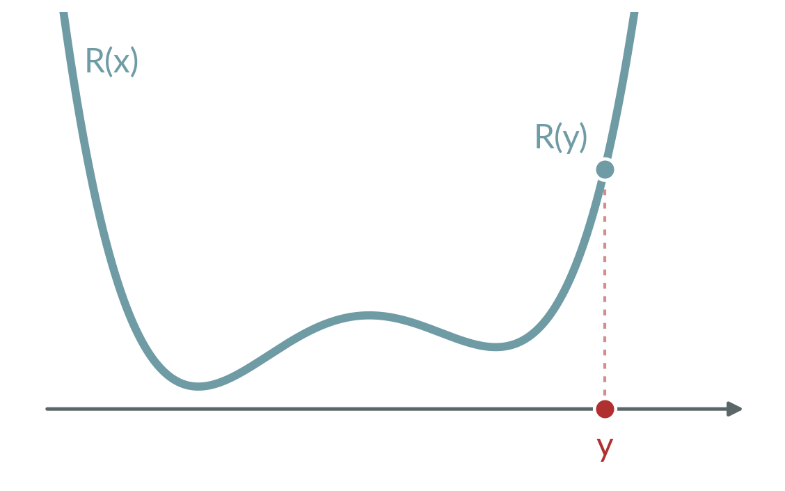
[Moreau 1962, 1965]
Proximal Operators
\text{prox}_{\lambda R}(y) ~\triangleq~ \underset{x}{\arg\min} ~ \tfrac12 \|x-y\|_2^2 + \lambda R(x)
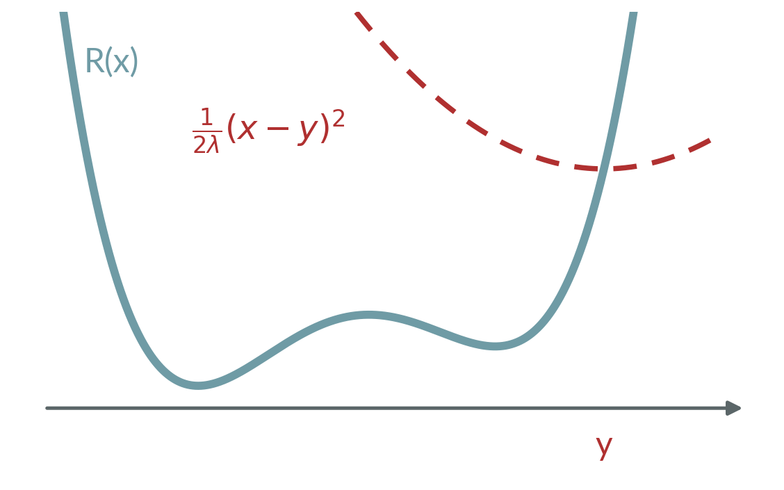
[Moreau 1962, 1965]
Proximal Operators
\text{prox}_{\lambda R}(y) ~\triangleq~ \underset{x}{\arg\min} ~ \tfrac12 \|x-y\|_2^2 + \lambda R(x)
\(\text{prox}_\lambda R (y) \to \arg\min R(x)\)
when \(\lambda \to \infty\)
Proximal Operators
\text{prox}_{\lambda R}(y) ~\triangleq~ \underset{x}{\arg\min} ~ \tfrac12 \|x-y\|_2^2 + \lambda R(x)
\(\text{prox}_\lambda R (y) = y\)
when \(\lambda = 0 \)
Proximal Operators
\(R(x) = \|x\|_1\)
\(R(x) = \|\nabla x\|_1\)
\(R(x) = \iota_C(x)\)
soft-thresholding
projection onto \(C\)
TV denoising
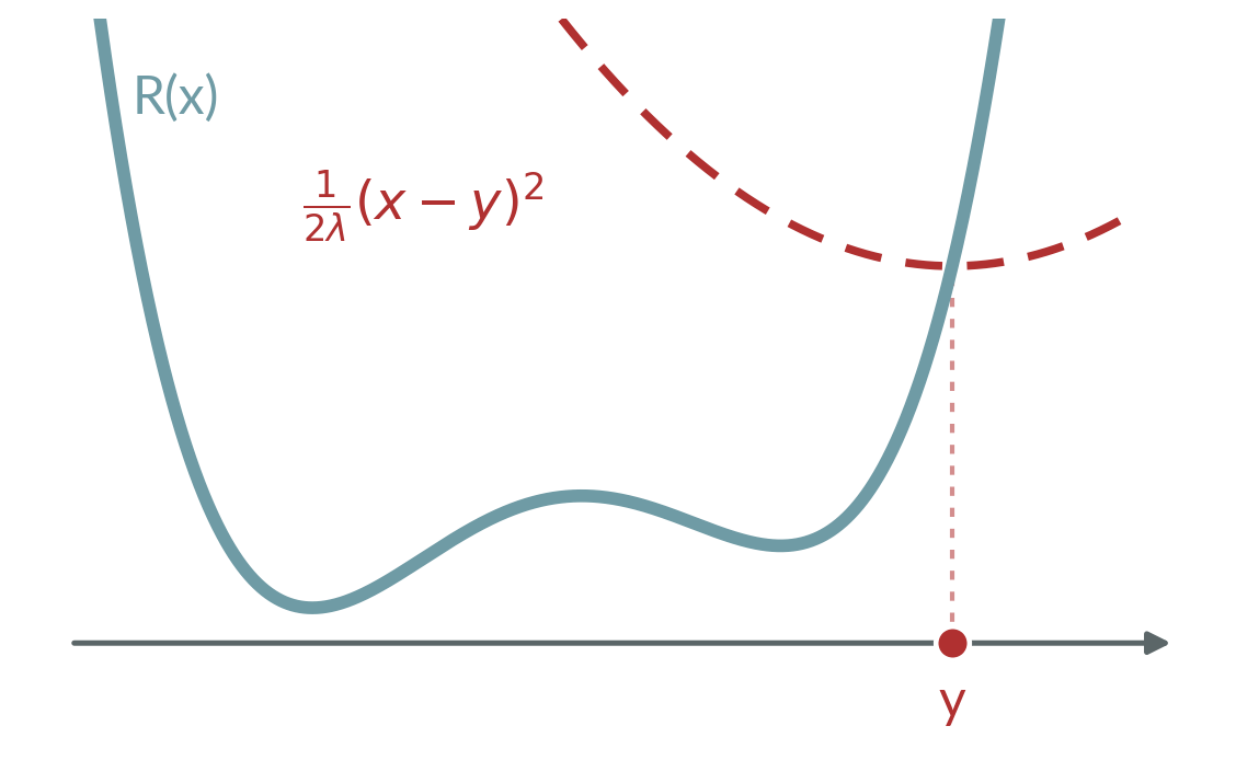
\text{prox}_{\lambda R}(y) ~\triangleq~ \underset{x}{\arg\min} ~ \tfrac12 \|x-y\|_2^2 + \lambda R(x)
Proximal Operators
\(R(x) = \|x\|_1\)
\(R(x) = \|\nabla x\|_1\)
\(R(x) = \iota_C(x)\)
soft-thresholding
projection onto \(C\)
TV denoising
\text{prox}_{\lambda R}(y) ~\triangleq~ \underset{x}{\arg\min} ~ \tfrac12 \|x-y\|_2^2 + \lambda R(x)
\underset{x}{\arg\min} ~ \tfrac12 \|x-y\|_2^2 + \underbrace{\|Wx\|_1}_{R(x)}
A Bayesian Perspective
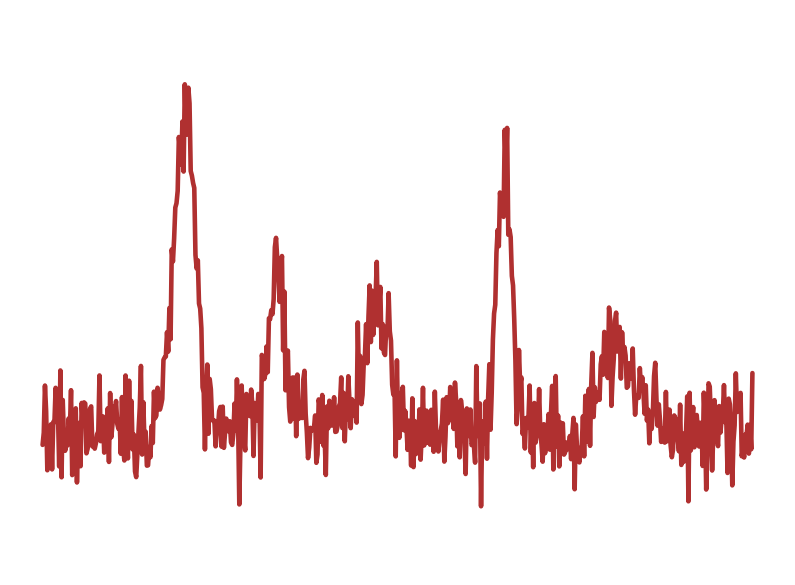
\(= \underset{x}{\arg\max} ~~~ p(y|x)p_x(x)\)
\(= \underset{x}{\arg\min} ~ -\log p(y|x) - \log p_x(x)\)
\(= \underset{x}{\arg\min} ~ \frac{1}{2\sigma^2} \|y-x\|^2_2 - \log p_x(x)\)
\(= \text{prox}_{-\sigma^2\log p_x}(y)\)
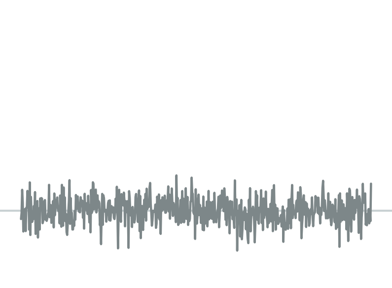
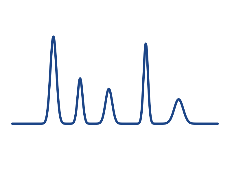
=
+
\(x\sim p_x\)
\(y = x + z\)
\(z\sim \mathcal N(0,\sigma^2 I)\)
\(\hat{x} = \underset{x}{\arg\max} ~ p(x|y)\)
Maximum a
Posteriori
estimator
MAP
A Bayesian Perspective
\(\underset{x}{\arg\min} ~ \frac1{2\sigma^2} \|y-x\|^2_2 - \log p_x(x)\)
\(= \text{prox}_{-\sigma^2\log p_x}(y)\)
observation
model of the world
\(y\)
\(p_x\)
\(\text{prox}_{-\sigma^2 \log p_x}(y)\)
\(R(x)\): regularizer
\(\underbrace{{\qquad}}{}\)
MAP(x|y):
A Bayesian Perspective
observation
model of the world
\(y\)
\(p_x\)
\(\text{prox}_{-\log p_x}(y)\)
Can we learn functions \(\hat{f}:\mathbb R^d\to\mathbb R\) from data \(x\sim p_x\) so that
\(\hat{f} = \text{prox}_R\) and \(R \to -\sigma^2\log p_x\)?
\(\underset{x}{\arg\min} ~ \frac1{2\sigma^2} \|y-x\|^2_2 - \log p_x(x)\)
\(= \text{prox}_{-\sigma^2\log p_x}(y)\)
\(R(x)\): regularizer
\(\underbrace{{\qquad}}{}\)
MAP(x|y):
Yes, enabling ...
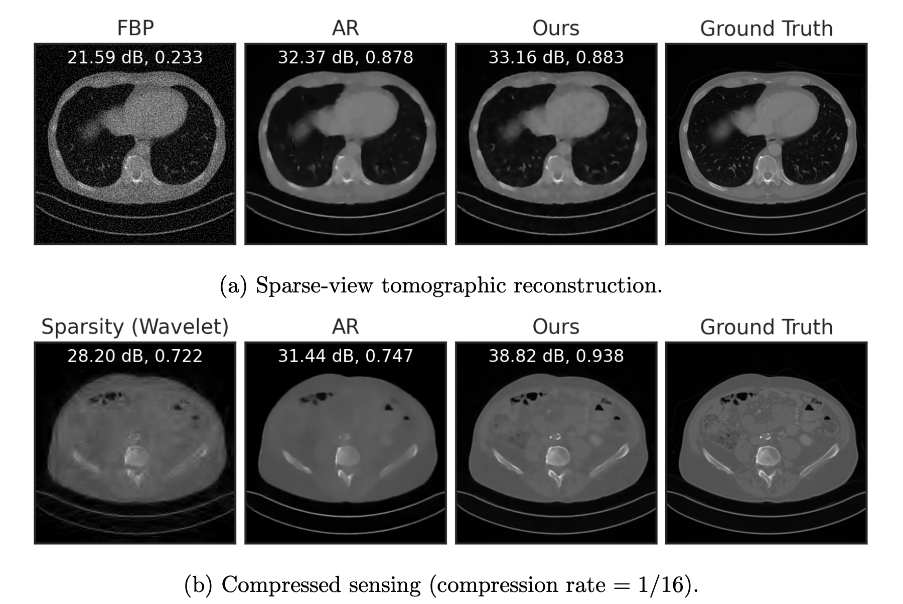
Inverse Problems
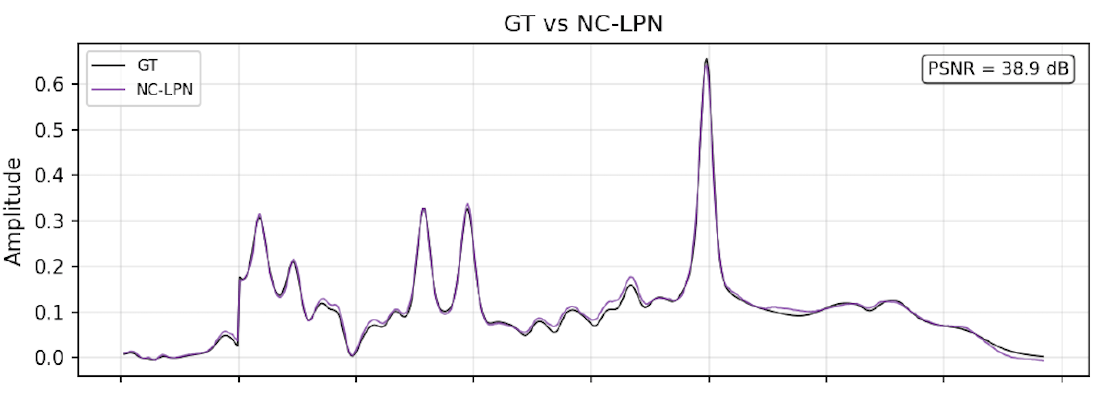
Outlier Detection
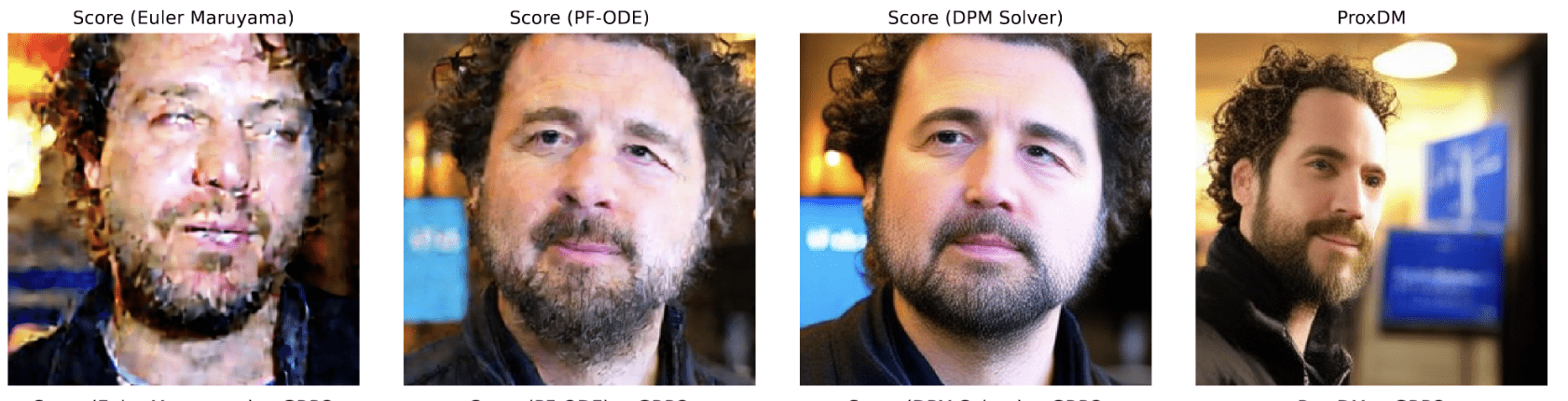
"A man with curly hair and a beard, wearing a dark jacket, stands indoors..."
Sampling
Can we learn functions \(\hat{f}:\mathbb R^d\to\mathbb R\) from data \(x\sim p_x\) so that
\(\hat{f} = \text{prox}_R\) and \(R \to -\sigma^2\log p_x\)?
Part I: Obtaining learned proximal operators
Part III: Sampling with learned proximals
Part II: Solving inverse problems
Can we learn functions \(\hat{f}:\mathbb R^d\to\mathbb R\) from data \(x\sim p_x\) so that
\(\hat{f} = \text{prox}_R\) and \(R \to -\sigma^2\log p_x\)?
Theorem [Fang, Buchanan, S.]
Let \(f: \mathbb R^d\to\mathbb R^d\) be a network : \(f_\theta (x) = \nabla \psi_\theta (x)\),
where \(\psi_\theta : \mathbb R^d \to \mathbb R,\) convex and differentiable.
Then,
1. Existence of regularizer
\(\exists ~R: \mathbb R^d \to \mathbb R\) not necessarily convex : \(f_\theta(x) \in \text{prox}_{R}(x),\)
2. Computability
We can compute \(R(x)\) by solving a convex problem
What functions are proximals?
see also (Gribonval & Nikolova, 2020)
Part I: Obtaining learned proximal operators
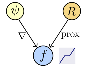
How do we obtain \(f = \text{prox}_{-\sigma^2\log p_x}\) from data?
Say \(y = x + z \), with \(z \sim \mathcal N(0,\sigma^2 I)\) and \(x\sim p_x\)
Denoisers: \(f(y) = \underset{f}{\arg\min} ~ \underset{x,z}{\mathbb E} \left[ \ell(f(y), x)\right]\)
Part I: Obtaining learned proximal operators
when \(\ell(y,x) = \|y- x\|^2_2\) \(\Rightarrow\) \(f(y) = \mathbb E[x|y]\)
Minimum mean squared estimators (MMSE)
\ell^\delta_\text{PM} (f(y),x) = 1- \exp\left( -\frac{\|f(y)-x\|_2^2}{\delta^2} \right)
Maximum a posteriori estimators
Part I: Obtaining learned proximal operators
Say \(y = x + z \), with \(z \sim \mathcal N(0,\sigma^2 I)\) and \(x\sim p_x\)
Denoisers: \(f(y) = \underset{f}{\arg\min} ~ \underset{x,z}{\mathbb E} \left[ \ell(f(y), x)\right]\)
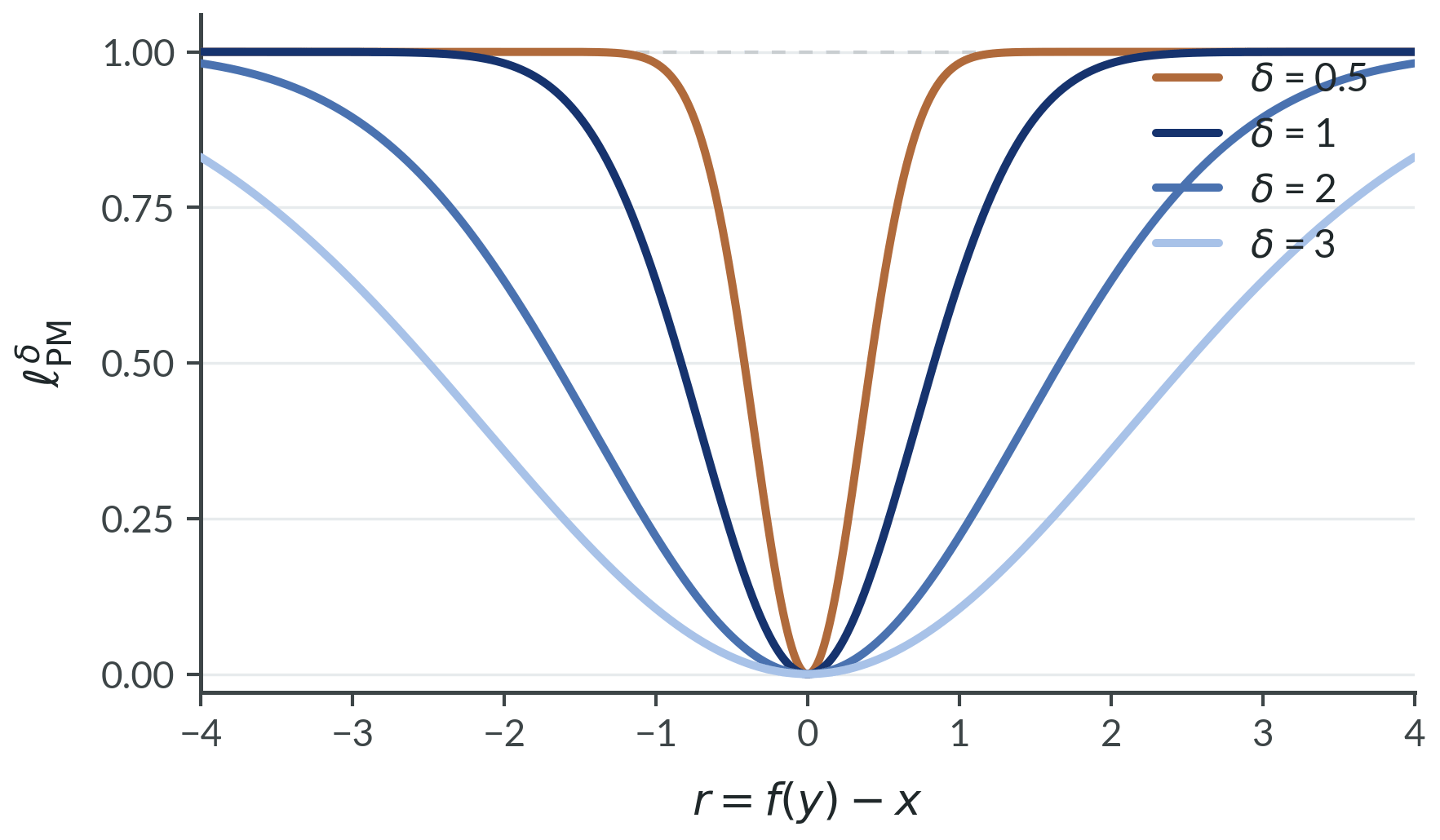
(informal)
Theorem [Fang, Buchanan, Díaz, S.]
f^* = ~\lim_{\delta \searrow 0}~ \mathop{\arg\min}\limits_{f:\,\text{measurable}} ~ \mathbb E_{x,z} \left[ \ell^\delta_\text{PM}(f(y),x)\right] = \text{prox}_{-\sigma^2\log p_x}
\text{Sample } y= x+z,~ \text{ with } x \sim \text{Laplace}(0,1) \text{ and } z\sim \mathcal N(0,\sigma^2)
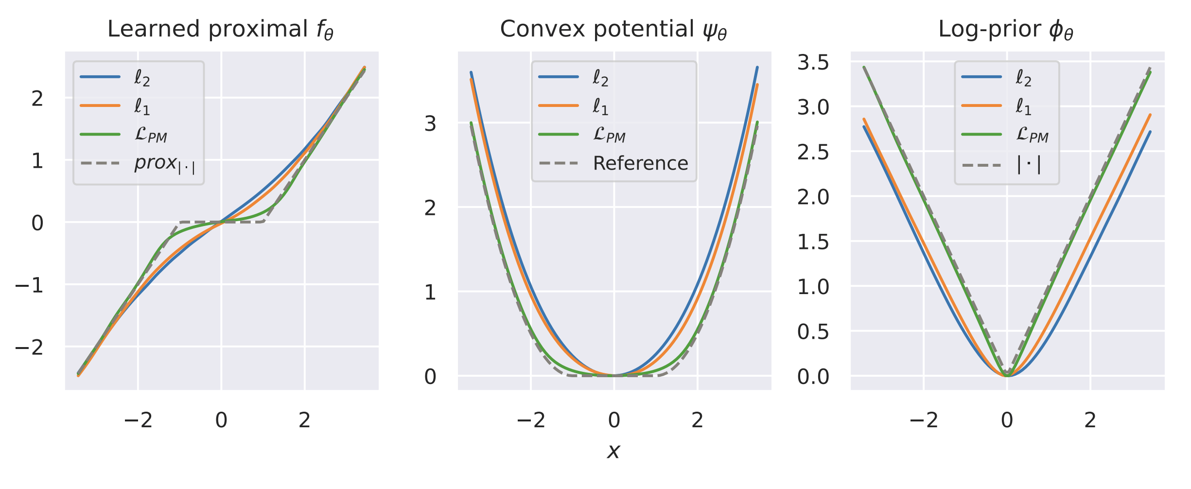
Example 0: recovering a prior
Part I: Obtaining learned proximal operators
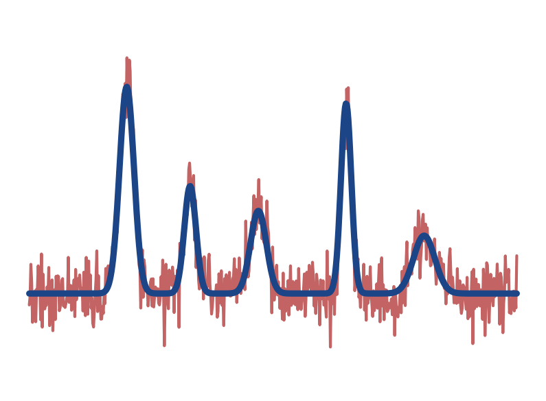
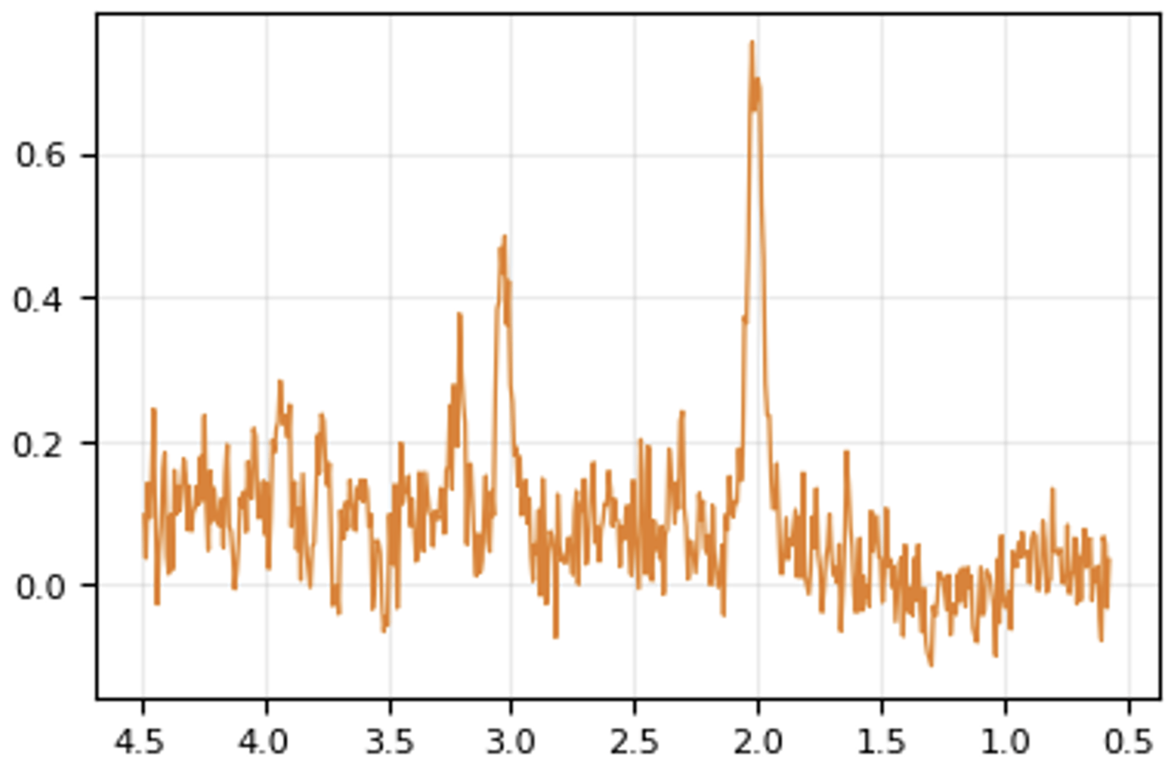
Example 1: learning a prior for MR Spectroscopy
Part I: Obtaining learned proximal operators
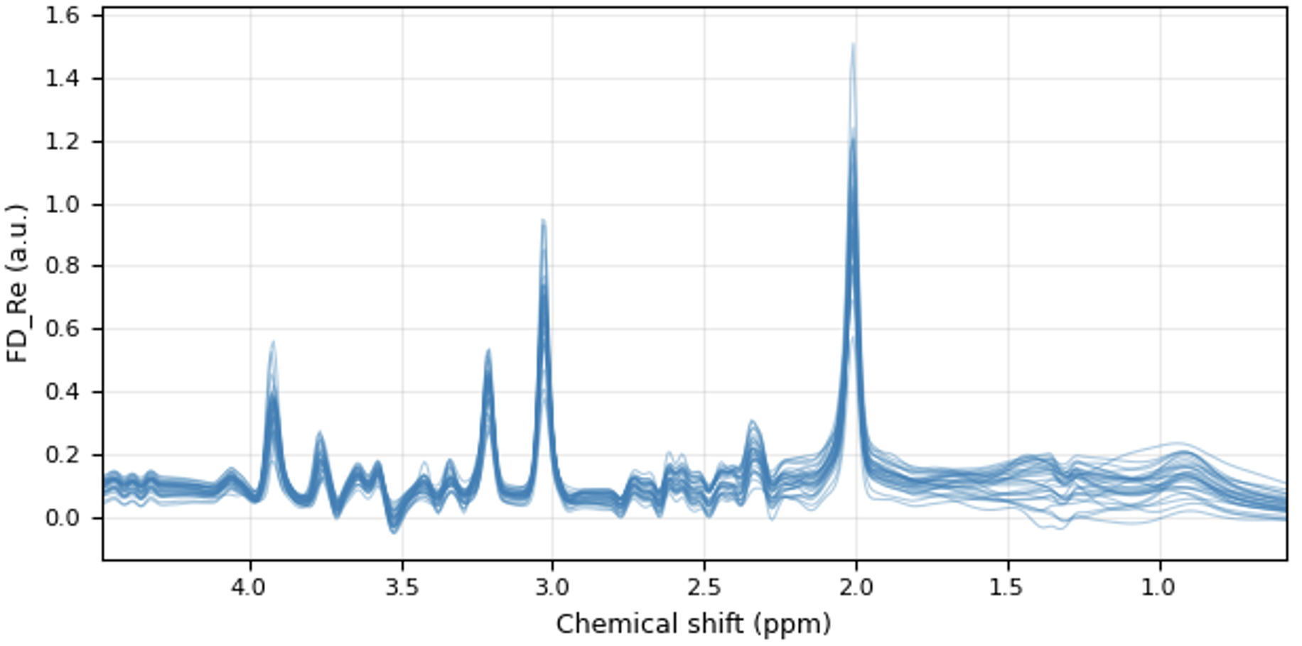
Part I: Obtaining learned proximal operators
Example 1: learning a prior for MR Spectroscopy
baseline
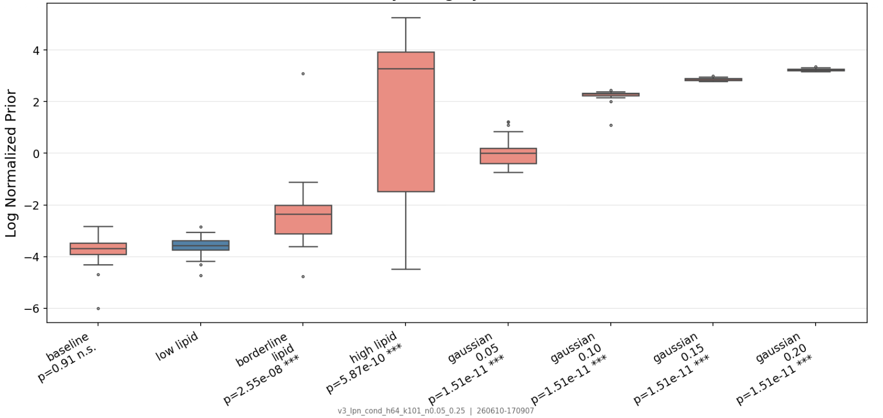
Part I: Obtaining learned proximal operators
Example 1: learning a prior for MR Spectroscopy
baseline
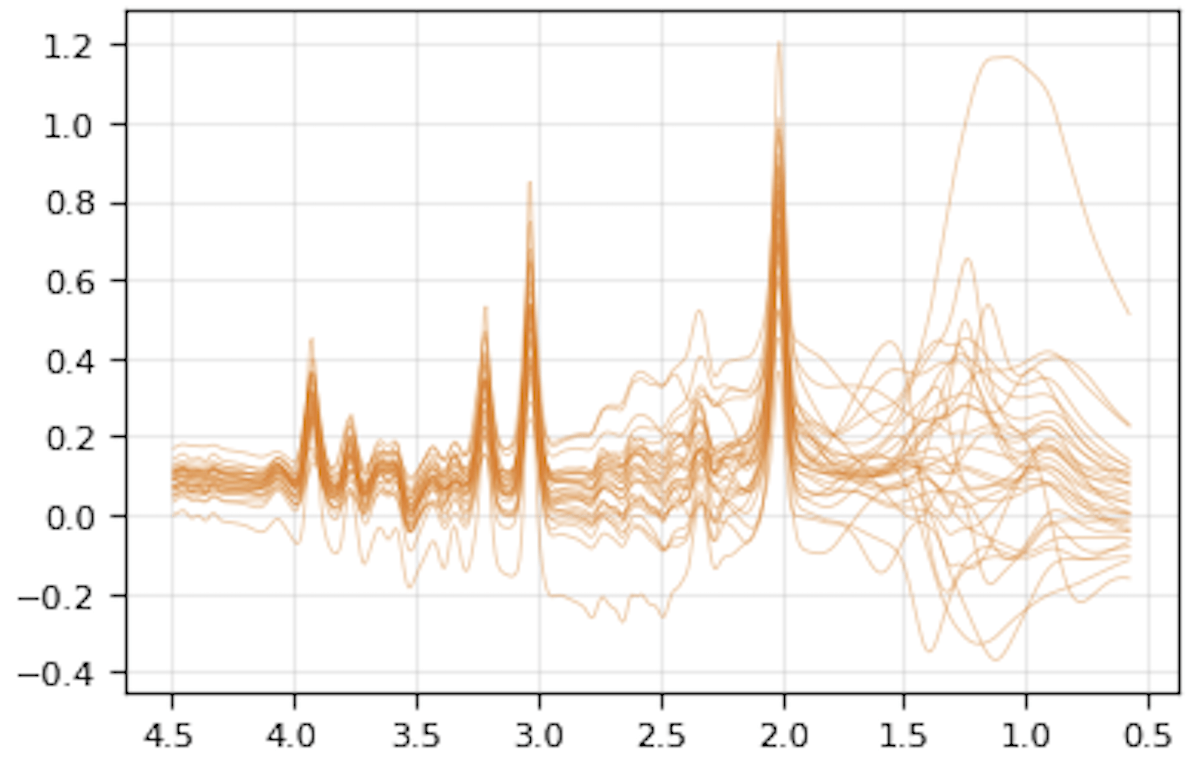
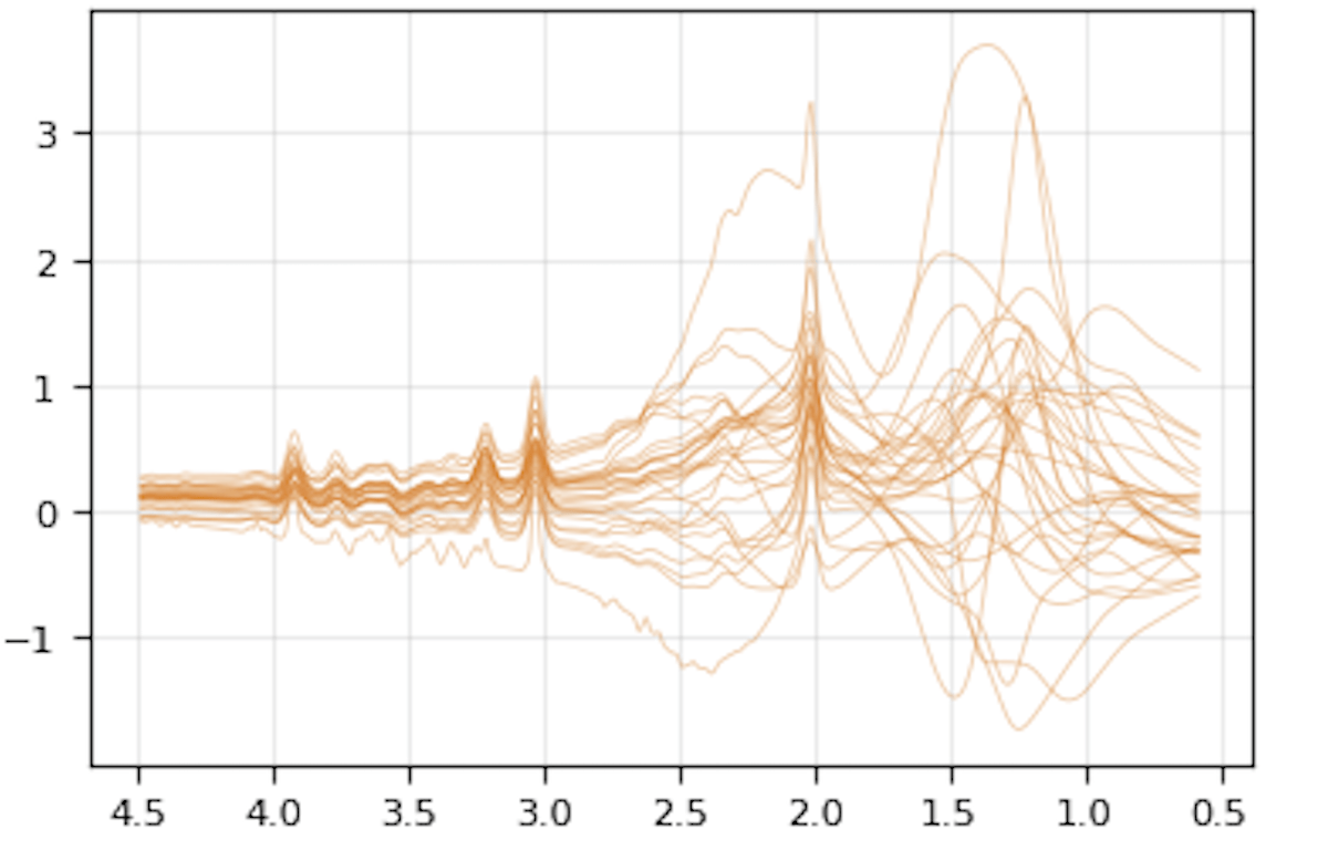
Part I: Obtaining learned proximal operators
Example 1: learning a prior for MR Spectroscopy
baseline
Part I: Obtaining learned proximal operators
Part III: Sampling with learned proximals
Part II: Solving inverse problems
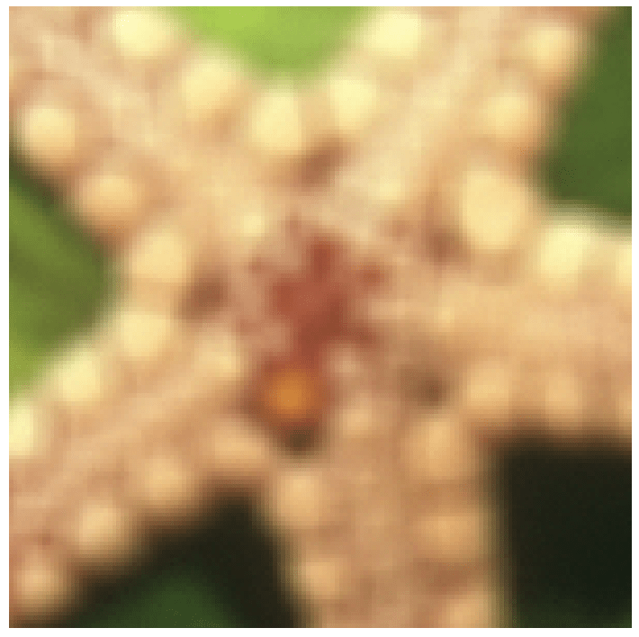
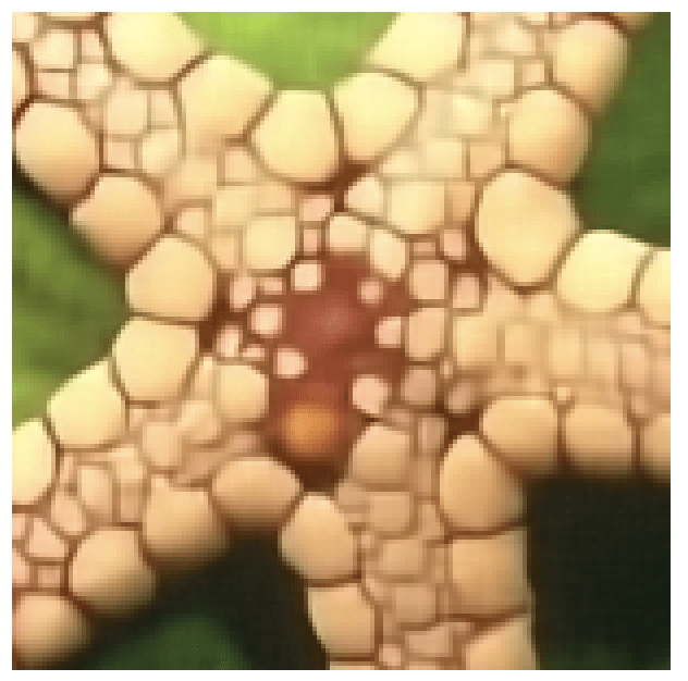
Part II: Solving inverse problems
\hat x = \arg\min_x \frac 12 \| y - A x \|^2_2 + R(x)
[Romano, Y., Elad, M., & Milanfar, P. (2017).]
Part II: Solving inverse problems
Unrolled Iteration (implicit priors)
\hat x = \arg\min_x \frac 12 \| y - A x \|^2_2 + R(x)
\( x^{k+1} = {\hat{f}} \left(x^k - \eta A^\top(A(x^k)-y)\right) \)
- Plug and Play
-
Neumann Networks
[Venkatakrishnan et al., 2013;
Zhang et al., 2017b;
Meinhardt et al., 2017;
Zhang et al., 2021;
Kamilov et al., 2023b;
Terris et al., 2023;
Hurault, Leclaire & Papadakis, 2022;
Vert, Kenta, et al., 2026]
[Gilton, Ongie, Willett, 2019]
-
Many other variations ...
Part II: Solving inverse problems
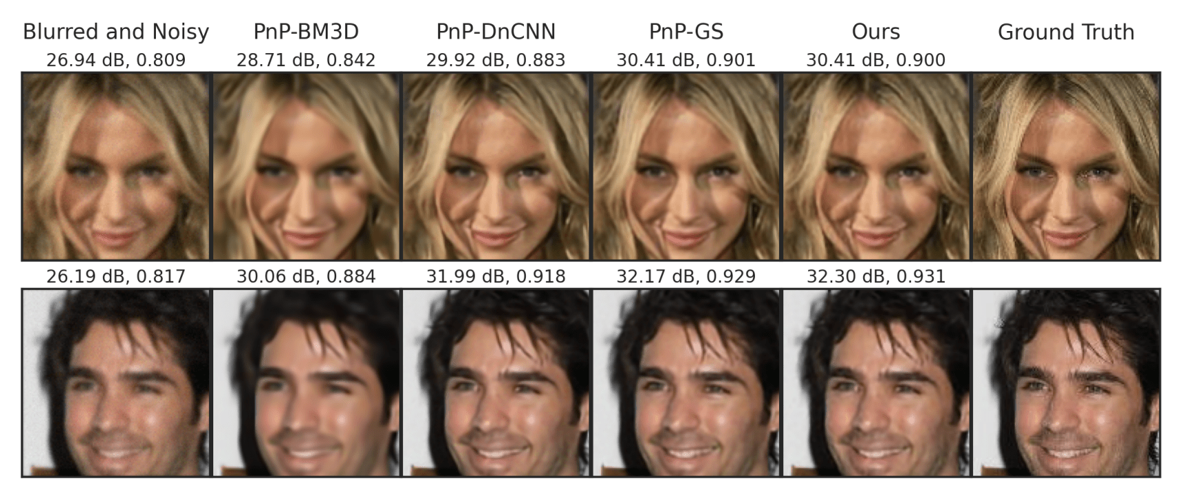
Learned-Proximal Gradient Descent
\hat x = \arg\min_x \frac 12 \| y - A x \|^2_2 + R(x)
\( x^{k+1} = {\hat{f}}_\text{LPN} \left(x^k - \eta A^\top(A(x^k)-y)\right) \)
Learned proximal networks trained with Proximal Matching
Part II: Solving inverse problems
Learned-Proximal Gradient Descent
\( x^{k+1} = {\hat{f}}_\text{LPN} \left(x^k - \eta A^\top(A(x^k)-y)\right) \)
Part II: Solving inverse problems
Learned-Proximal Gradient Descent
\( x^{k+1} = {\hat{f}}_\text{LPN} \left(x^k - \eta A^\top(A(x^k)-y)\right) \)
Theorem (PGD with Learned Proximal Networks)
x^{k+1} = \hat{f}_{\hat R} \left(x^k - \eta A^\top(Ax^k - y)\right)
Let \(f_\theta = \text{prox}_{\hat{R}} \) be an LPN (smooth activations, invertible, bounded step-size)
\text{Then } \exists x^* : \lim_{k\to\infty} x^k = x^* \text{ and }
f_\theta(x^* - \eta A^\top(Ax^*-y)) = x^*
(Analogous results hold for ADMM)
Part I: Obtaining learned proximal operators
Part III: Sampling with learned proximals
Part II: Solving inverse problems
Part III: Sampling with learned proximals
Goal: Draw samples \(x\sim p_x\)

Part III: Sampling with learned proximals
\(t\)
[Song et al, 2019][Ho et al, 2020]
dx_t = - \left[ x_t + 2 \nabla \ln p_t(x_t)\right] dt + \sqrt{2} dw_t
Diffusion process:
Part III: Sampling with learned proximals
x_{\color{red}k-1} = x_{\color{blue}k} + \gamma_k\left[ \frac12 x_{\color{blue}k}+ \nabla \ln p_{t_{\color{blue}k}}(x_{\color{blue}k}) \right] + \sqrt{\gamma_k}z_k
Forward discretization:
(DDPM)
[Ho et al, 2020]dx_t = - \left[ x_t + 2 \nabla \ln p_t(x_t)\right] dt + \sqrt{2} dw_t
Part III: Sampling with learned proximals
x_{\color{red}k-1} = x_{\color{blue}k} + \gamma_k\left[ \frac12 x_{\color{red}k-1}+ \nabla \ln p_{t_k}(x_{\color{red}k-1}) \right] + \sqrt{\gamma_k}z_k
Backward discretization:
Forward discretization:
(DDPM)
[Ho et al, 2020]x_{\color{red}k-1} = x_{\color{blue}k} + \gamma_k\left[ \frac12 x_{\color{blue}k}+ \nabla \ln p_{t_{\color{blue}k}}(x_{\color{blue}k}) \right] + \sqrt{\gamma_k}z_k
dx_t = - \left[ x_t + 2 \nabla \ln p_t(x_t)\right] dt + \sqrt{2} dw_t
Part III: Sampling with learned proximals
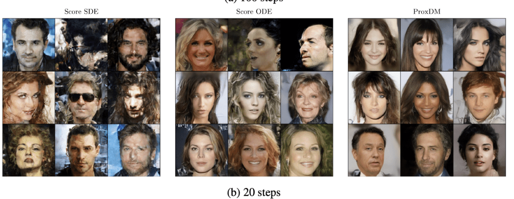
Backward discretization:
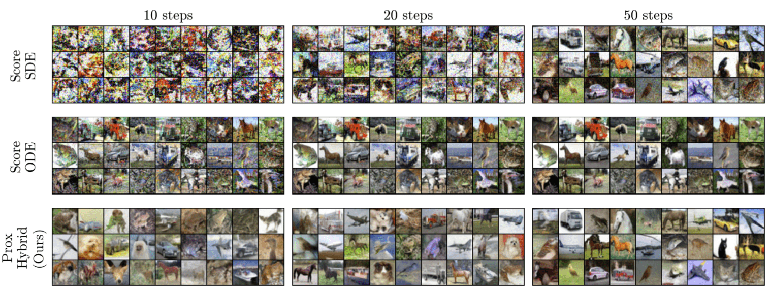
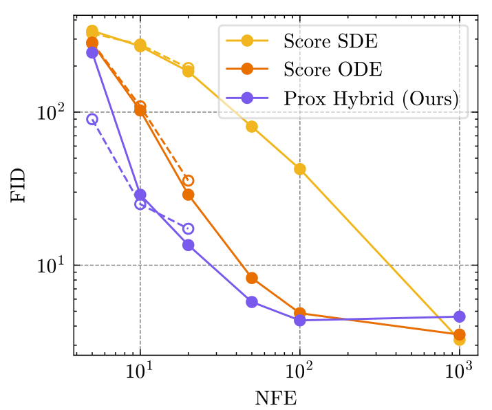
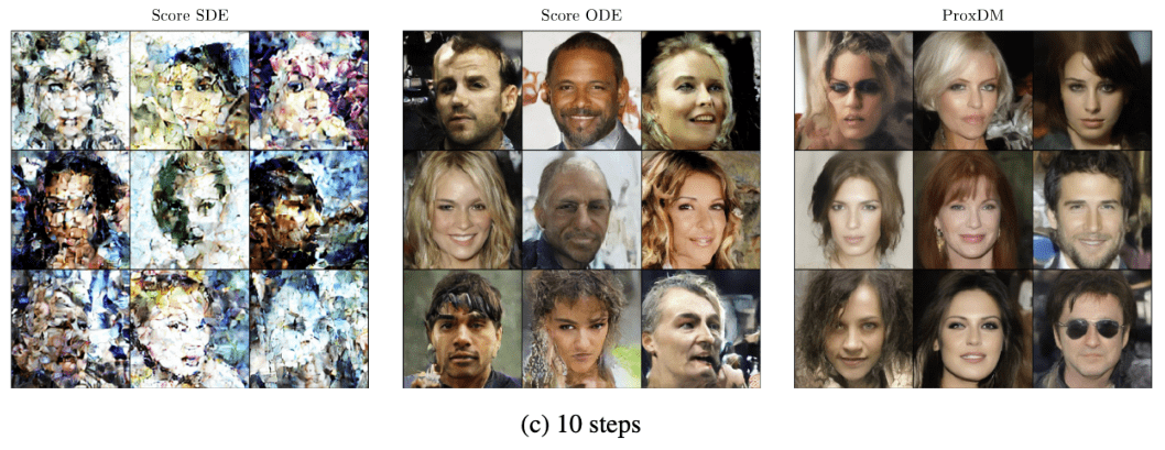
(ProxDM)
x_{\color{red}k-1} = x_{\color{blue}k} + \gamma_k\left[ \frac12 x_{\color{blue}k}+ \nabla \ln p_{t_{\color{blue}k}}(x_{\color{blue}k}) \right] + \sqrt{\gamma_k}z_k
Forward discretization:
(DDPM)
dx_t = - \left[ x_t + 2 \nabla \ln p_t(x_t)\right] dt + \sqrt{2} dw_t
[Ho et al, 2020]x_{k-1} = \text{prox}_{-\alpha_k \ln p_{t_{k-1}}}\left[ \frac{2}{2-\gamma_k}\left( x_k + \sqrt{\gamma_k} z_k \right) \right]


- Bounded moments: \(\mathbb E \|X\|^2 \lesssim d\), \(\mathbb E \|\nabla \ln p_t (X)\|^2 \lesssim dL^2\)
- Smoothness: \(\ln p_t\) has \(L\)-Lipschitz gradient and \(H\)-Lipschitz Hessian
- Step-size: \( \gamma \lesssim 1/L \)
- Regularity conditions: technical but common
Theorem [Fang, Díaz, Buchanan, S.]
(informal)
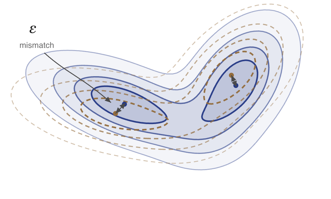
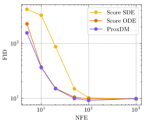
ProxDM requires \(N\gtrsim {d/\sqrt{\epsilon}}\)
To achieve \(\text{KL}(\text{target}||\text{sample})\leq \epsilon\)
DDPM requires \(N\) is \(\mathcal O( d/\epsilon)\) (vanilla) or \(\mathcal O(d^{3/4}/\sqrt{\epsilon})\) if accelerated
[Chen et al, 2022][Wu et al, 2024]
Part III: Sampling with learned proximals
Sampling acceleration
Probability Flows and ODEs (e.g. DDIM) [Song et al 2020, Chen et al, 2023, ...]
DPM-solver [Lu et al 2022]
Higher-order solvers [Wu et al, 2024, ... ]
Accelerations of different kinds [Song et al, 2023, Chen et al, 2025, ... ]
Benefits of backward discretization of ODEs/SDEs
Optimization [Rockafellar, 1976], [Beck and Teboulle, 2015] ...
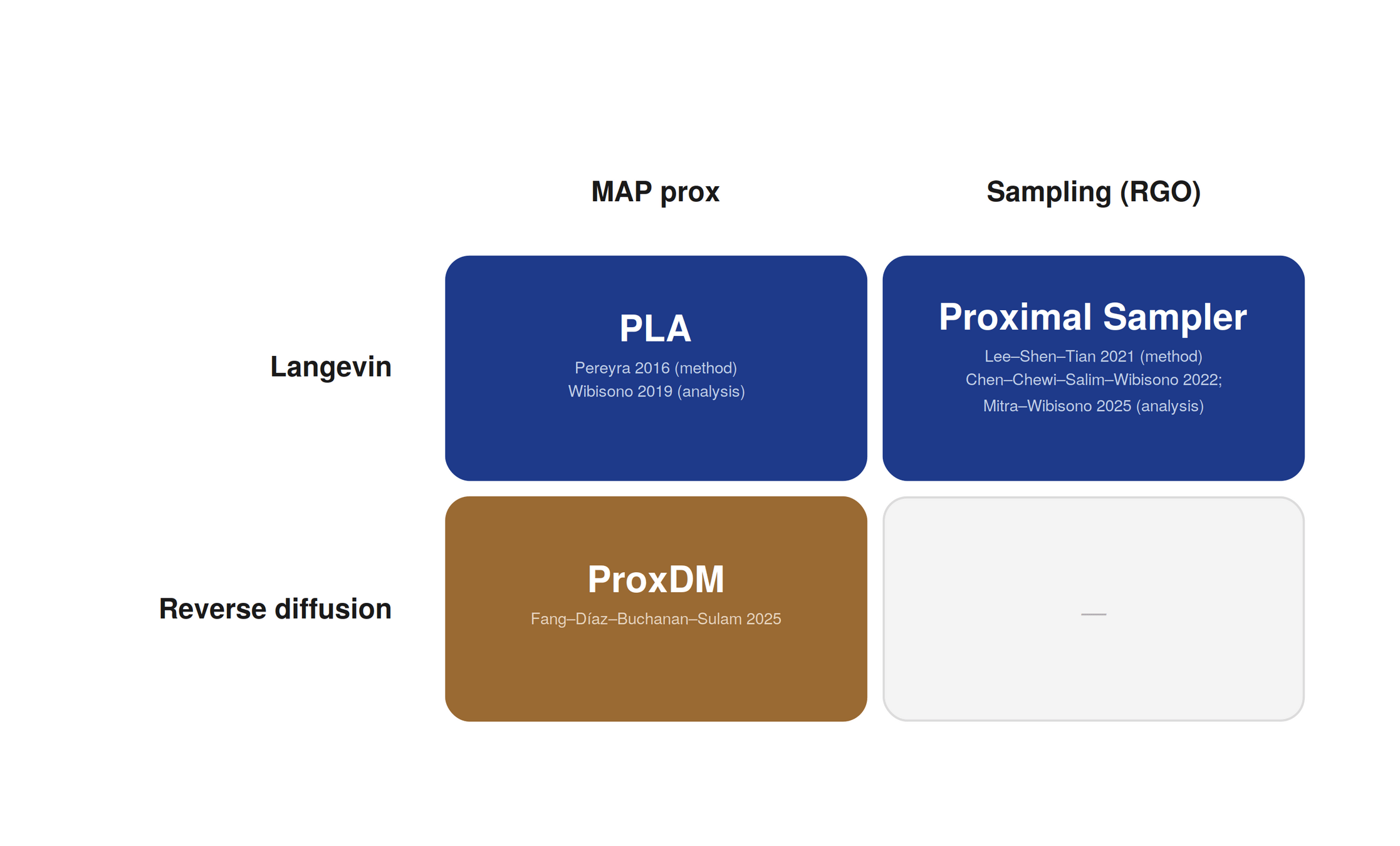
Langevin Dynamics: PLA [Bernton 2018, Pereyra 2016, Wibisono 2019, Durmus et al 2018]
Forward-backward in space of measures [Chen et al 2018, Wibisono, 2025, Chen et al 2026]
Part III: Sampling with learned proximals
Part III: Sampling with learned proximals
Part III: Sampling with learned proximals
Part III: Sampling with learned proximals
\(x \sim p_{x_0|\text{signal}}\)
e.g. \(\text{signal}=\)
"A woman with long blonde hair and a black top stands against a neutral background. She wears a delicate necklace. The image is a portrait-style photograph with soft lighting."
dX_t = - \left[ X_t + 2 \nabla \ln p_t(X_t\mid {\color{brown}\text{signal}})\right] dt + \sqrt{2} dW_t
Diffusion process:
X_{k-1} = \text{prox}_{-\alpha_k \ln p_{k-1}(\cdot\mid{\color{brown}\text{signal})}}\left[ \frac{2}{2-\gamma_k}\left( X_k + \sqrt{\gamma_k} Z_k \right) \right]
Conditional ProxDM (ProxT2I)
Part III: Sampling with learned proximals
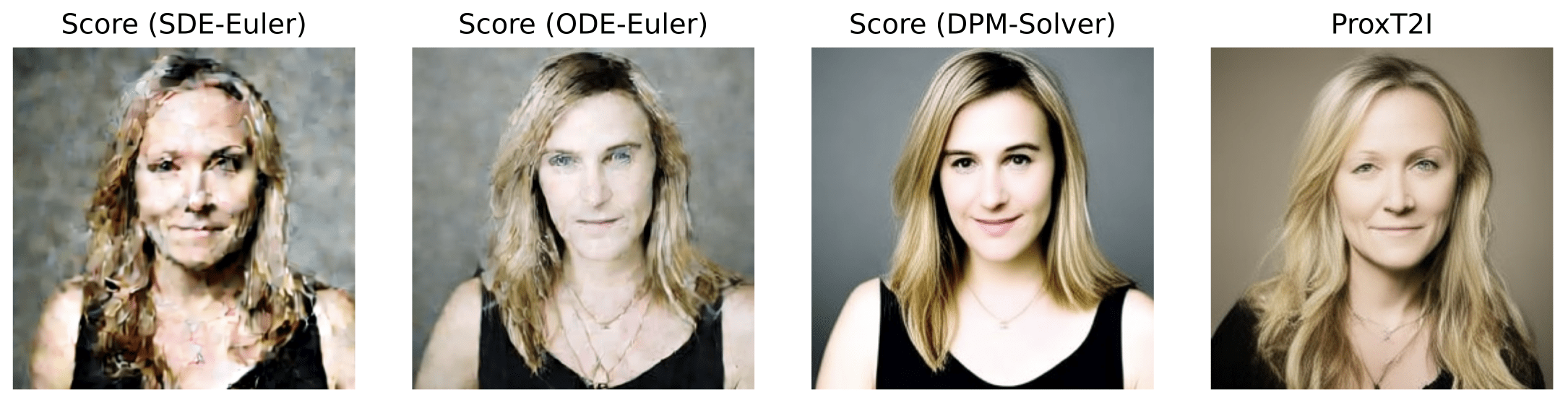
(10 steps)
e.g. \(\text{signal}=\)
"A woman with long blonde hair and a black top stands against a neutral background. She wears a delicate necklace. The image is a portrait-style photograph with soft lighting."
\(x \sim p_{x_0|\text{signal}}\)
Part III: Sampling with learned proximals
Part I: Obtaining learned proximal operators
Part III: Sampling with learned proximals
Part II: Solving inverse problems
Wrapping up
Sampling
Outlier Detection
Inverse Problems
Proximal Operators
Wrapping up
Constrained Optimization
Proximal Operators
Learned
Inverse Problems
Outlier Detection
"A man with curly hair and a beard, wearing a dark jacket, stands indoors..."
Sampling
- Flexible parametrizations for proximal operators
- Approximations for log-densities
- Many open problems (constraint sampling, UQ, ...)
Zhenghan Fang

Sam Buchanan
Mateo Díaz

Yuqing He
-
Fang et al, Learned Proximal Networks for Inverse Problems, ICLR 2024.
-
Fang et al, Beyond Scores: Proximal Diffusion Models, Neurips 2025.
-
Fang et al, ProxT2I: Efficient Reward-Guided Text-to-Image Generation via Proximal Diffusion, arXiv 2025.


Team
Appendix
Mathematical tractability vs Complexity
in a box
simpler models
more assumptions
any model
no assumptions
Denoiser
Linear models
Linear networks
Shallow
ReLU Networks
Just ask GPT
Learned Proximal Operators

Q2: How do we implement proximal diffusion models?
- How do we train so that \(f_\theta \approx \text{prox}_{-\ln p}\) ?
\( \text{prox}_{-\ln p}(Y) = \underset{X}{\arg\min} \frac12 \|X-Y\|^2_2 - \ln p(X) \)
\text{Let } Y = X+Z , \quad ~ X\sim p_0, ~~Z \sim \mathcal N(0,\sigma^2I)
\( = {\arg\max}~ p(X|Y) ~~~~ \text{(MAP)}\)
f_\theta = \arg\min_{f_\theta} \mathbb E \left[ {{\color{red}\ell} (f_\theta(Y),X)} \right]
\bullet ~~ {\ell (f_\theta(Y),X)} = \|f_\theta(Y) - X\|^2_2 ~~\implies~~ \mathbb E[X|Y] \text{ (MMSE)}
\bullet ~~ {\ell (f_\theta(Y),X)} = \|f_\theta(Y) - X\|_1 ~~\implies~~ \texttt{median}(p_{X|Y})
examples
Denoiser:
\text{Sample } Y= X+Z,~ \text{ with } X \sim \text{Laplace}(0,1) \text{ and } Z\sim \mathcal N(0,\sigma^2)
Example: recovering a prior
Q2: How do we implement proximal diffusion models?
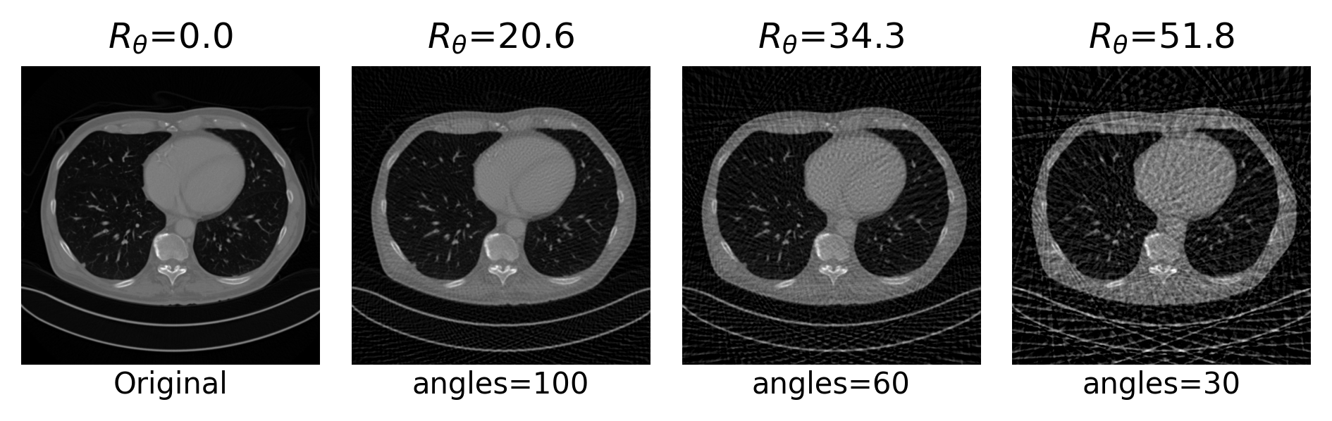
Example 2: a prior for CT
Aside 2: What (data-driven) functions are proxs?
Example 2: a prior for CT
Aside 2: What (data-driven) functions are proxs?
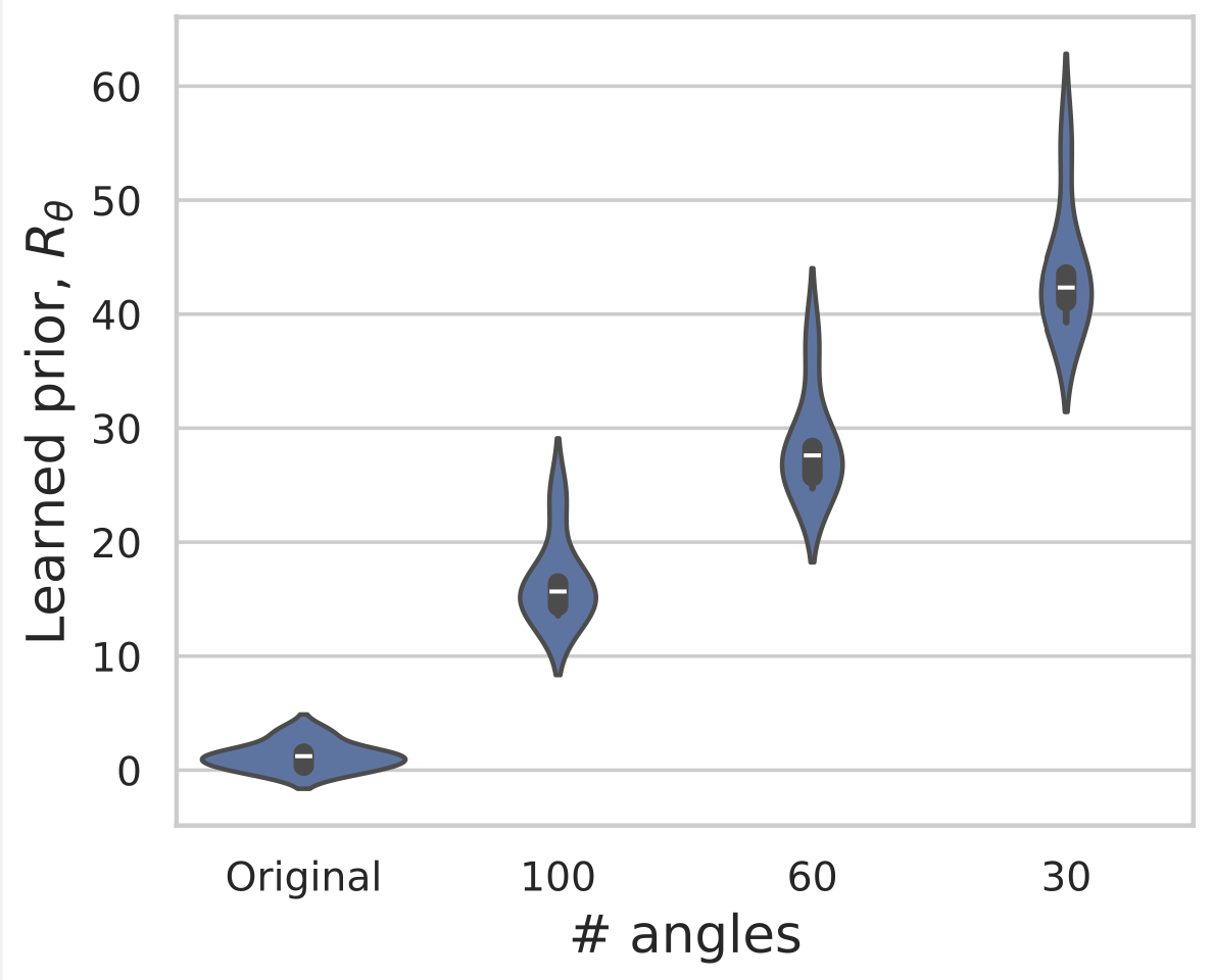
Example 2: a prior for CT
Aside 2: What (data-driven) functions are proxs?
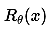
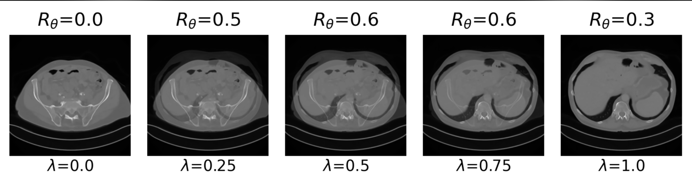
Example 2: a prior for CT
Aside 2: What (data-driven) functions are proxs?
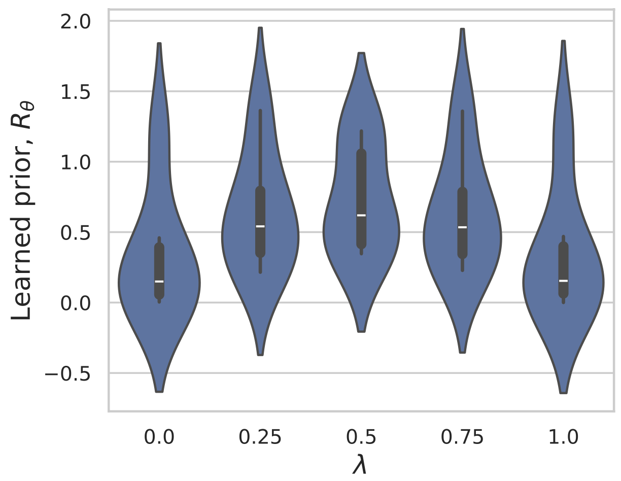
Example 2: a prior for CT
Aside 2: What (data-driven) functions are proxs?
Learned Proximal Networks
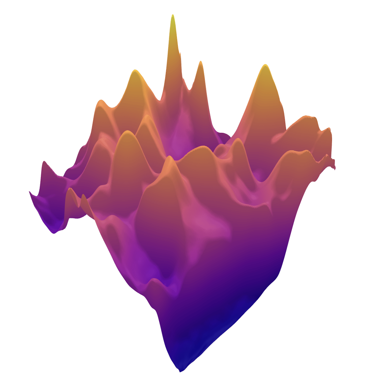
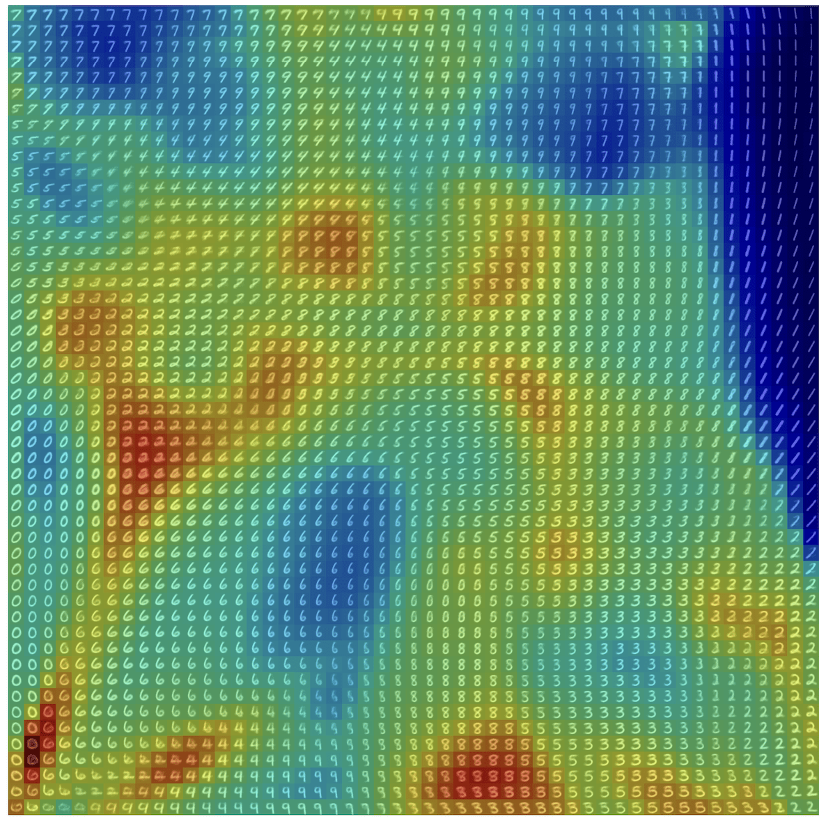
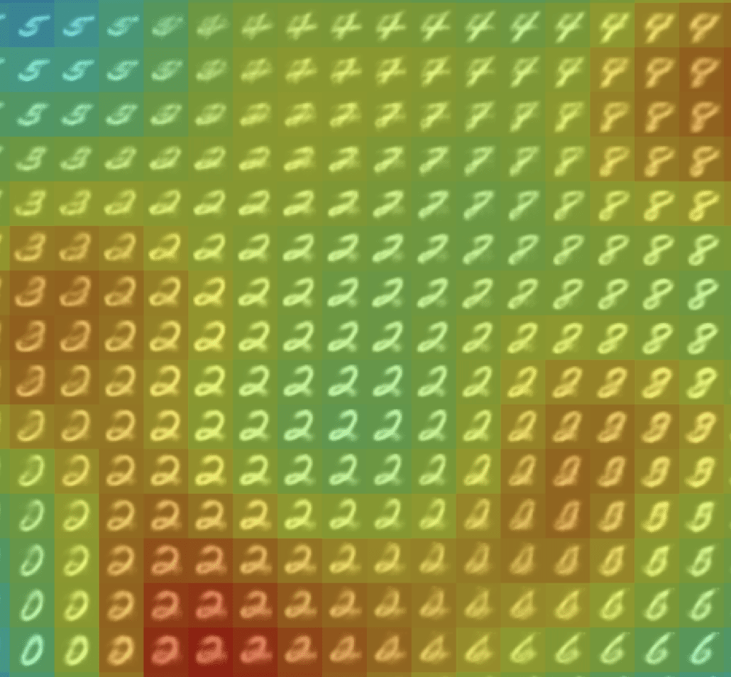
\(R(\tilde{x})\)
Example 2: priors for images
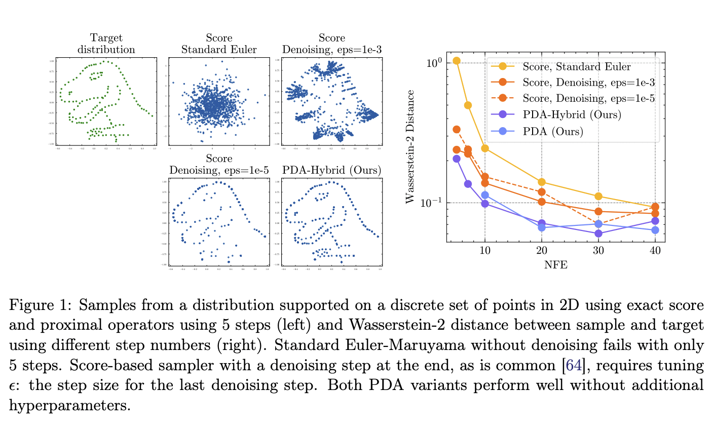
ProxDM Synthetic
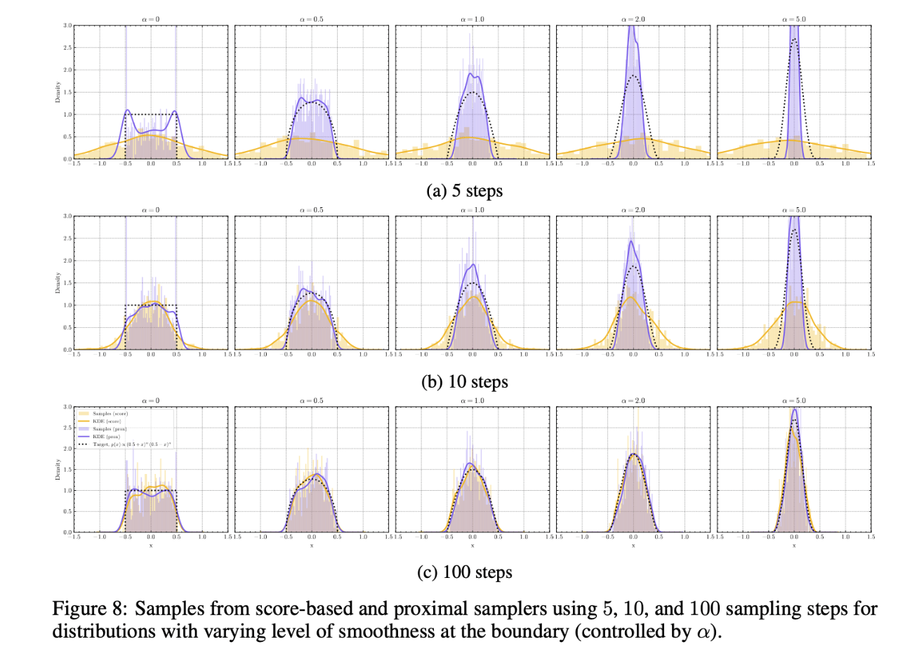
ProxDM Synthetic 2
Related Works
Learned Proximal Operators - SPS Webinar
By Jeremias Sulam