What's in my network?
Jeremias Sulam
On learned proximals and testing for explanations


Communications and Signal Processing Seminar
October 2024


"The biggest lesson that can be read from 70 years of AI research is that general methods that leverage computation are ultimately the most effective, and by a large margin. [...] Seeking an improvement that makes a difference in the shorter term, researchers seek to leverage their human knowledge of the domain, but the only thing that matters in the long run is the leveraging of computation. [...]
We want AI agents that can discover like we can, not which contain what we have discovered."
The Bitter Lesson, Rich Sutton 2019

What did my model learn?
PART I
Inverse Problems
PART II
Image Classification
Inverse Problems
y = A x^* + v
measurements
\hat x = \arg\min_x \frac 12 \| y - A x \|^2_2 + R(x)
reconstruction
Inverse Problems
y = A x^* + v
measurements
\hat x = \arg\min_x \frac 12 \| y - A x \|^2_2 + R(x)
reconstruction
= \arg\min_x ~-\log p(y|x) - \log p(x)
= \arg\max_x~ p(x|y)
\text{MAP estimate when }R(x) \propto -~p_x(x):\text{ prior}

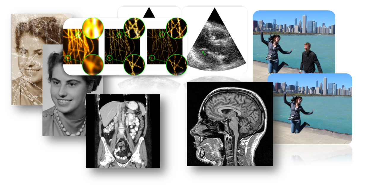
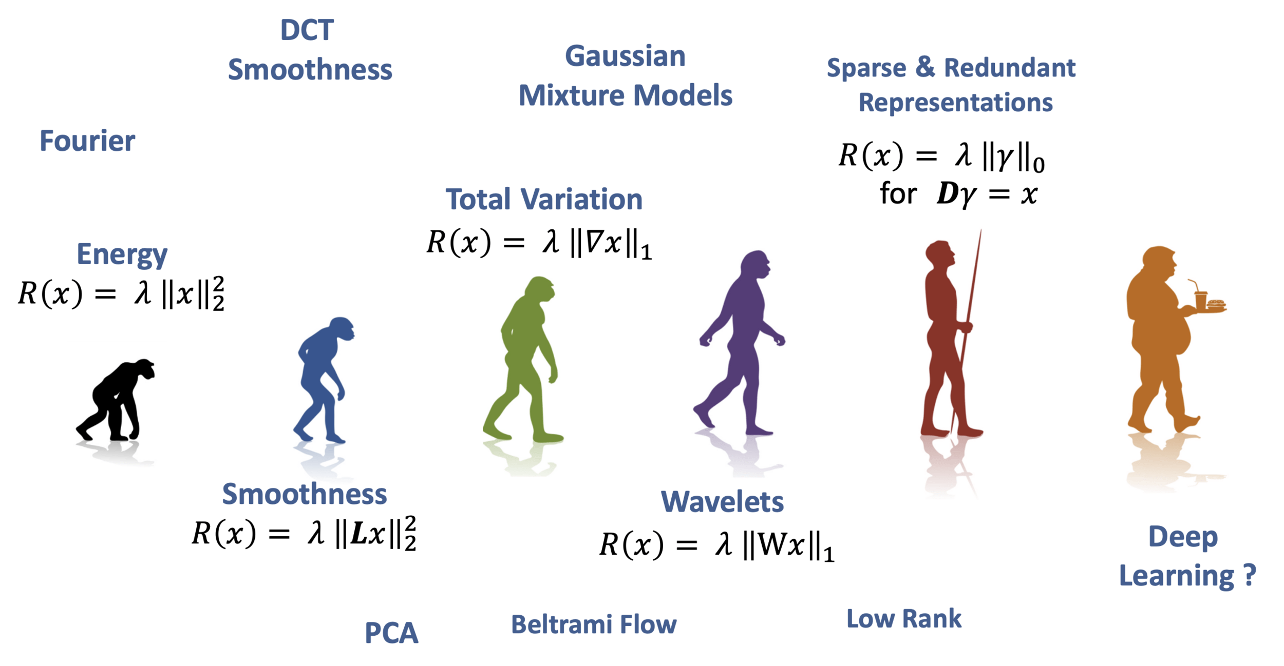
Image Priors
Deep Learning in Inverse Problems
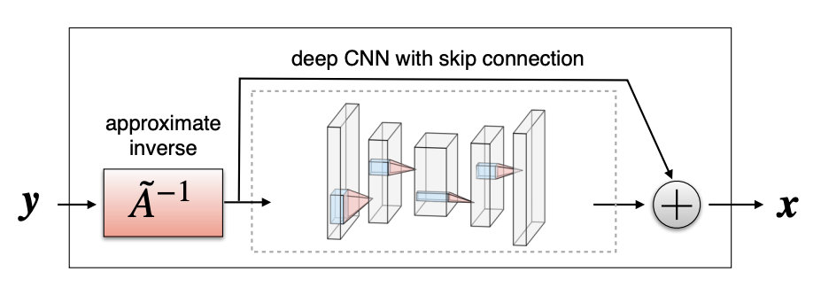
Option A: One-shot methods
Given enough training pairs \({(x_i,y_i)}\) train a network
\(f_\theta(y) = g_\theta(A^+y) \approx x\)
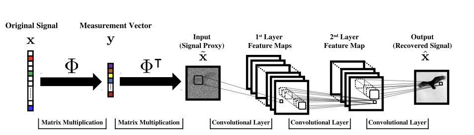
[Mousavi & Baraniuk, 2017]
[Ongie, Willet, et al, 2020]
Deep Learning in Inverse Problems
Option B: data-driven regularizer
\hat x = \arg\min_x \frac 12 \| y - A x \|^2_2 + {\color{Green}\hat R_\theta(x)}
- Priors as critics
[Lunz, Öktem, Schönlieb, 2020] and others ..
\displaystyle \hat R_\theta(x) = \arg\min_{R_\theta\in
\mathcal H} ~ \mathbb E_{x\sim p_x}[R(x)] - \mathbb E_{x\sim q }[R(x)]
- via MLE
[Ye Tan, ..., Schönlieb, 2024], ...
- RED
[Romano et al, 2017] ...
- Generative Models
[Bora et al, 2017] ...
\displaystyle \hat R_\theta(x) = \mathbb 1_{[\exist z : G(z)=x]}
Deep Learning in Inverse Problems
Option C: Implicit Priors
\hat x = \arg\min_x \frac 12 \| y - A x \|^2_2 + R(x)
Proximal Gradient Descent: \( x^{t+1} = \text{prox}_R \left(x^t - \eta A^T(Ax^t-y)\right) \)
\text{prox}_R \left( u \right) = \arg\min_x \frac 12 \|u - x\|_2^2 + R(x)
\text{prox}_R \left( u \right) = \texttt{MAP}(X|u), \qquad u = x + v
... a denoiser
Deep Learning in Inverse Problems
\hat x = \arg\min_x \frac 12 \| y - A x \|^2_2 + R(x)
any latest and greatest NN denoiser
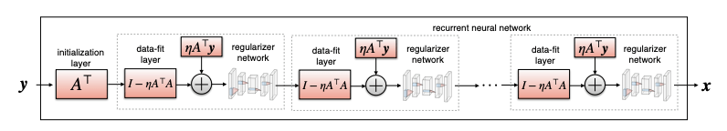
[Venkatakrishnan et al., 2013; Zhang et al., 2017b; Meinhardt et al., 2017; Zhang et al., 2021; Kamilov et al., 2023b; Terris et al., 2023]
[Gilton, Ongie, Willett, 2019]
Proximal Gradient Descent: \( x^{t+1} = {\color{red}f_\theta} \left(x^t - \eta A^T(A(x^t)-y)\right) \)
Option C: Implicit Priors
Question 1)
When will \(f_\theta(x)\) compute a \(\text{prox}_R(x)\) ? and for what \(R(x)\)?
Deep Learning in Inverse Problems
\(\mathcal H_\text{prox} = \{f : \text{prox}_R~ \text{for some }R\}\)
\(\mathcal H = \{f: \mathbb R^n \to \mathbb R^n\}\)
Question 1)
When will \(f_\theta(x)\) compute a \(\text{prox}_R(x)\) ? and for what \(R(x)\)?
Question 2)
Can we estimate the "correct" prox?
Deep Learning in Inverse Problems
\text{prox}_R : R(x) = -\log p_x(x)
\(\mathcal H_\text{prox} = \{f : \text{prox}_R~ \text{for some }R\}\)
\(\mathcal H = \{f: \mathbb R^n \to \mathbb R^n\}\)
\hat x = \arg\min_x \frac 12 \| y - A x \|^2_2 + R(x)
= \arg\min_x ~-\log p(y|x) - \log p(x)
= \arg\max_x~ p(x|y)
Interpretable Inverse Problems
Question 1)
When will \(f_\theta(x)\) compute a \(\text{prox}_R(x)\) ?
Theorem [Gibonval & Nikolova, 2020]
\( f(x) \in \text{prox}_R(x) ~\Leftrightarrow \exist ~ \text{convex l.s.c.}~ \psi: \mathbb R^n\to\mathbb R : f(x) \in \partial \psi(x)~\)
Interpretable Inverse Problems
Question 1)
When will \(f_\theta(x)\) compute a \(\text{prox}_R(x)\) ?
\(R(x)\) need not be convex
Theorem [Gibonval & Nikolova, 2020]
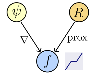
Learned Proximal Networks
Take \(f_\theta(x) = \nabla \psi_\theta(x)\) for convex (and differentiable) \(\psi_\theta\)
\( f(x) \in \text{prox}_R(x) ~\Leftrightarrow \exist ~ \text{convex l.s.c.}~ \psi: \mathbb R^n\to\mathbb R : f(x) \in \partial \psi(x)~\)
Interpretable Inverse Problems
Question 1)
When will \(f_\theta(x)\) compute a \(\text{prox}_R(x)\) ?
\(R(x)\) need not be convex
Learned Proximal Networks
Take \(f_\theta(x) = \nabla \psi_\theta(x)\) for convex (and differentiable) \(\psi_\theta\)
\( f(x) \in \text{prox}_R(x) ~\Leftrightarrow \exist ~ \text{convex l.s.c.}~ \psi: \mathbb R^n\to\mathbb R : f(x) \in \partial \psi(x)~\)
Theorem [Gribonval & Nikolova, 2020]
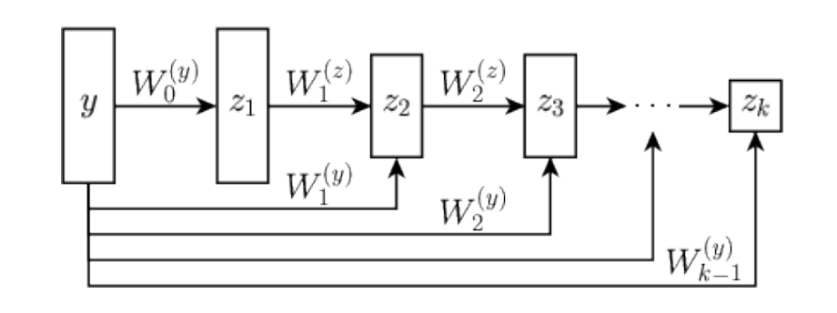
\psi_\theta : \mathbb R^d \to \mathbb R \text{ given by } \psi_\theta(y) = w^Tz_K + b \text{ and }
z_1 = g(H_1y+b_1), \quad z_k = g(W_k z_{k-1} + H_ky + b_k ), k\in [2,K]
g: \text{convex, non-decreasing, } W_k \text{ and }w_K: \text{non-negative entries}.
\left( \psi_\theta(x,\alpha) = \psi_\theta(x) + \frac \alpha 2 \|x\|^2_2 \right)
Interpretable Inverse Problems
If so, can you know for what \(R(x)\)?
R_\theta(x) = \langle {\color{red}\hat{f}^{-1}_\theta(x)},x\rangle - \frac 12 \|x\|^2_2 - \psi_\theta( {\color{red}\hat{f}^{-1}_\theta(x)} )
[Gibonval & Nikolova]
Easy! \[{\color{grey}y^* =} \arg\min_{y} \psi(y) - \langle y,x\rangle {\color{grey}= \hat{f}_\theta^{-1}(x)}\]
Interpretable Inverse Problems
Question 2)
Could we have \(R(x) = -\log p_x(x)\)?
(we don't know \(p_x\)!)
\text{Let } y = x+v , \quad ~ x\sim p_x, ~~v \sim \mathcal N(0,\sigma^2I)
f_\theta = \arg\min_{f_\theta:\text{prox}} \mathbb E_{x,y} \left[ {\ell (f_\theta(y),x)} \right]
\bullet ~~ {\ell (f_\theta(y),x)} = \|f_\theta(y) - x\|^2_2 ~~\implies~~ \mathbb E[x|y] \text{ (MMSE)}
\bullet ~~ {\ell (f_\theta(y),x)} = \|f_\theta(y) - x\|_1 ~~\implies~~ \texttt{median}(p_{x|y})
i.e. \(f_\theta(y) = \text{prox}_R(y) = \texttt{MAP}(x|y)\)
Which loss function?
Interpretable Inverse Problems
i.e. \(f_\theta(y) = \text{prox}_R(y) = \texttt{MAP}(x|y)\)
Theorem (informal)
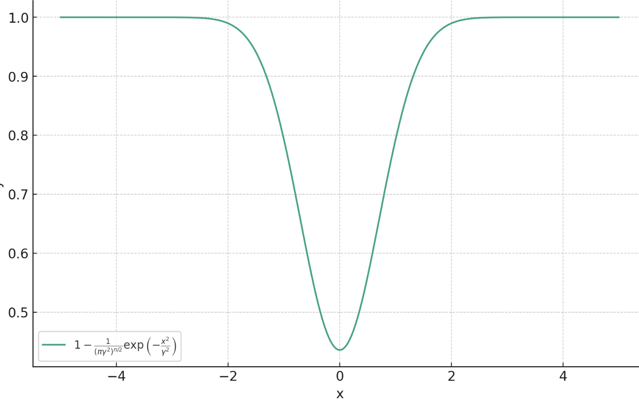
\hat{f}^* = \arg\min_{f} \lim_{\gamma \searrow 0}~ \mathbb E_{x,y} \left[ \ell^\gamma_\text{PM}(f_\theta(y),x)\right]
\hat{f}^*(y) = \arg\max_c p_{x|y}(c) = \text{prox}_{-\sigma^2\log p_x}(y)
\ell^\gamma_\text{PM} (f_\theta(y),x) = 1- \frac{1}{(\pi\gamma^2)^{n/2}} \exp\left( -\frac{\|f(y)-x\|_2^2}{\gamma} \right)
Proximal Matching Loss
\(\gamma\)
Question 2)
Could we have \(R(x) = -\log p_x(x)\)?
(we don't know \(p_x\)!)
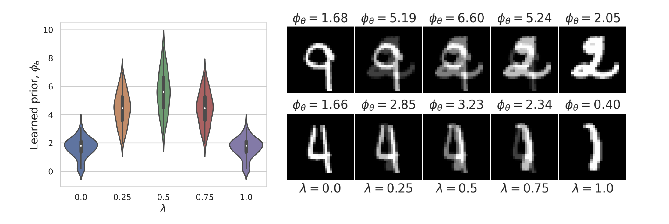
Learned Proximal Networks
\text{Sample } y = x+v,~ \text{ with } x \sim \text{Laplace}(0,1) \text{ and } v \sim \mathcal N(0,\sigma^2)
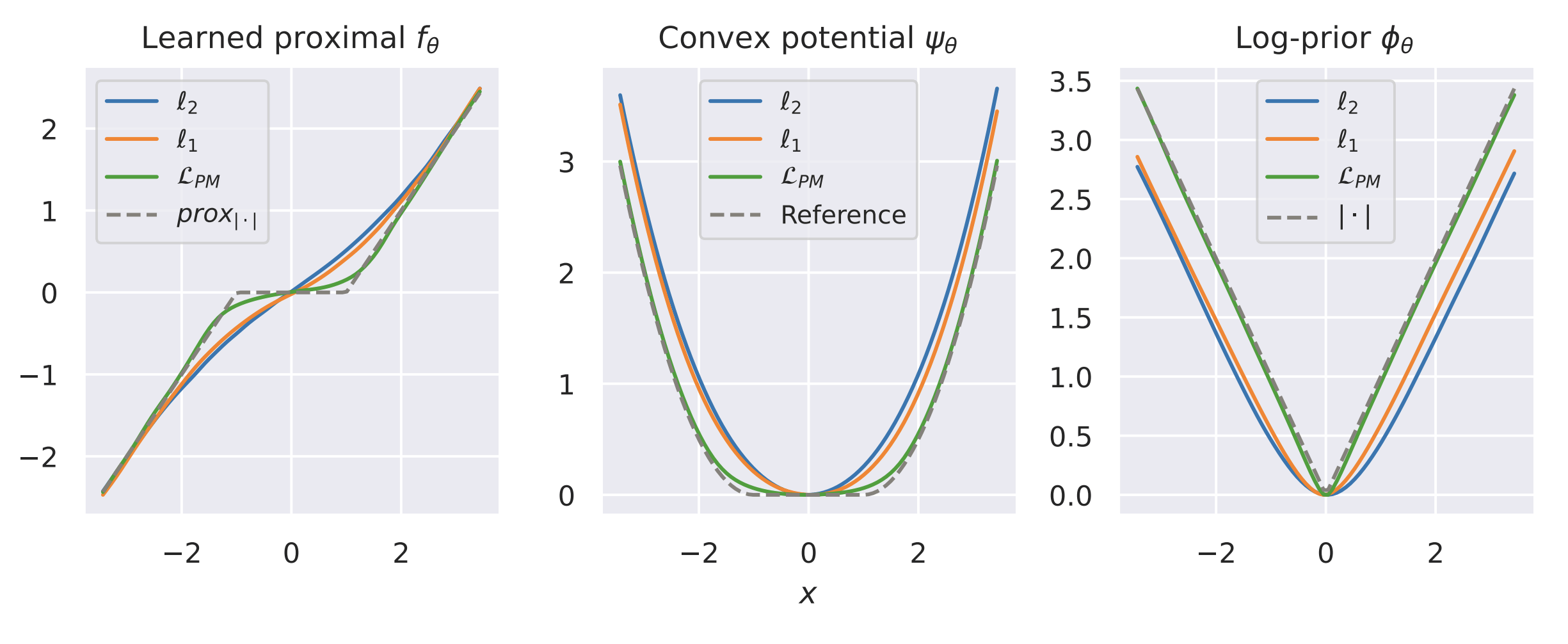
Example 1: recovering a prior
Learned Proximal Networks
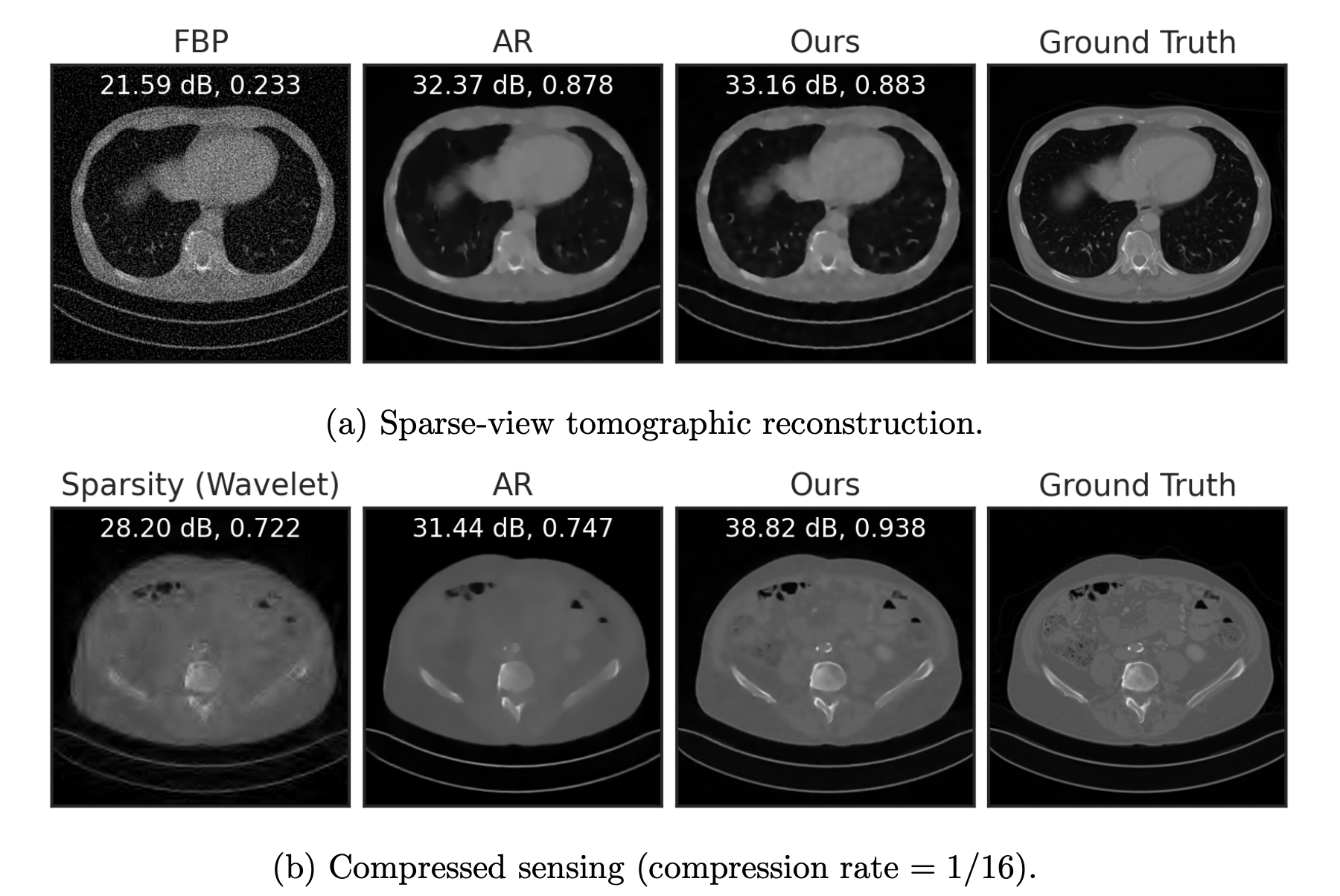
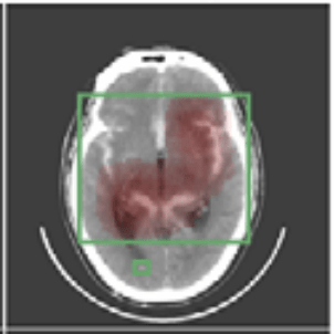
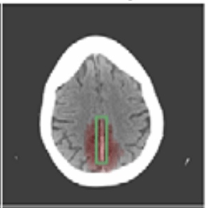
Example 2: a prior for CT
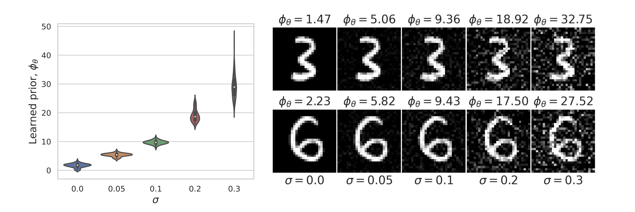
Learned Proximal Networks
Example 2: a prior for CT
Learned Proximal Networks
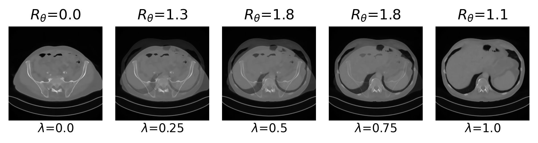
Example 2: a prior for CT
Learned Proximal Networks
Example 2: a prior for CT
Learned Proximal Networks
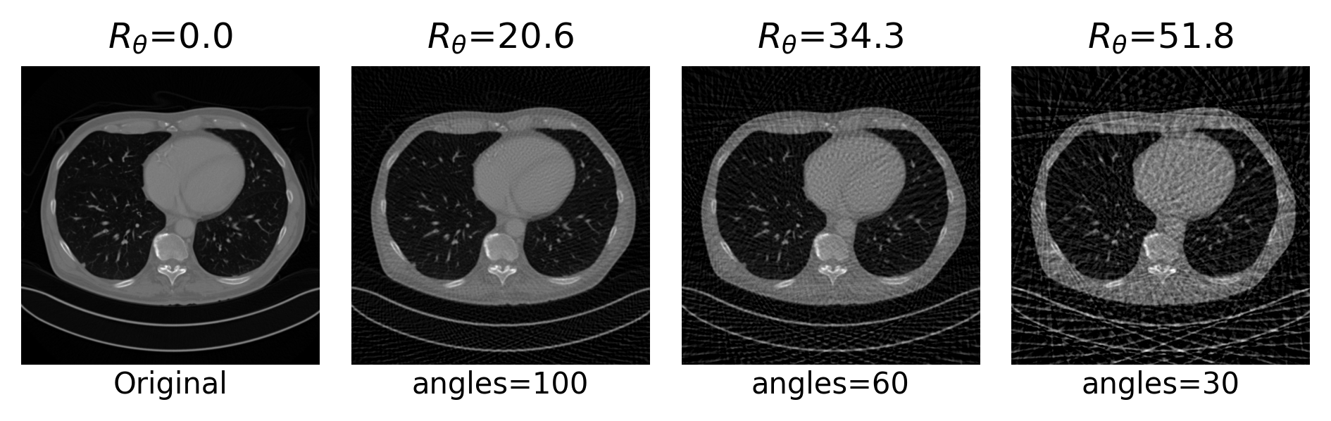
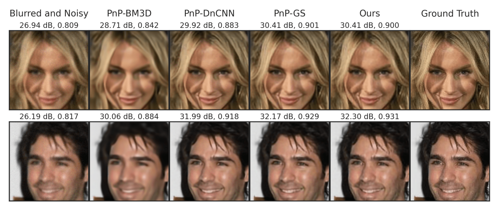
Example 2: priors for images
Learned Proximal Networks
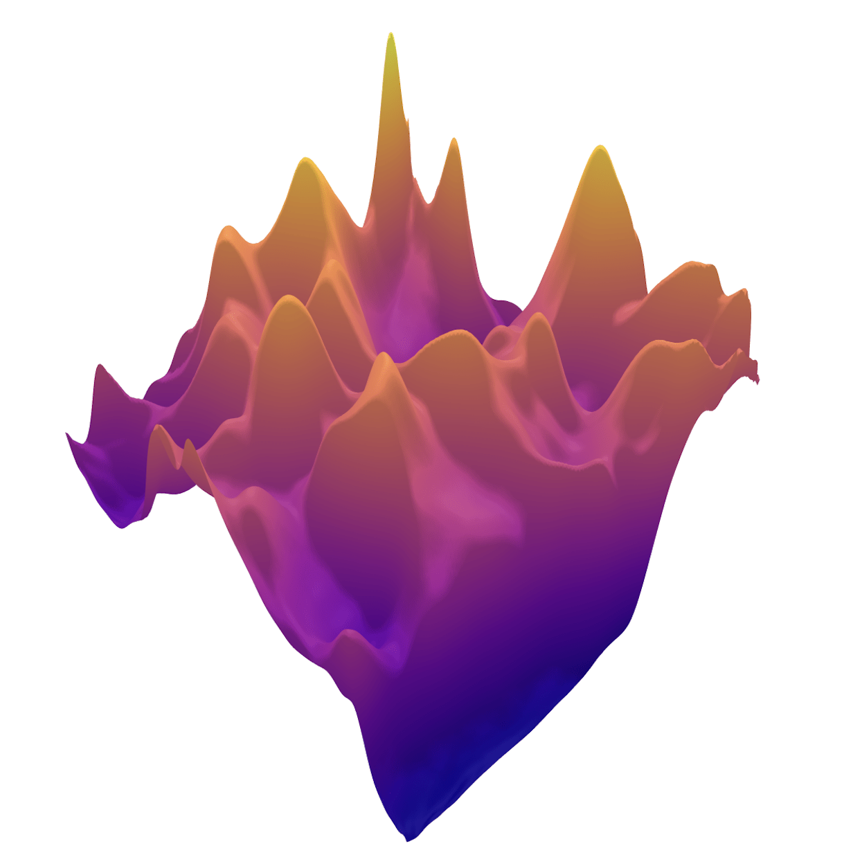
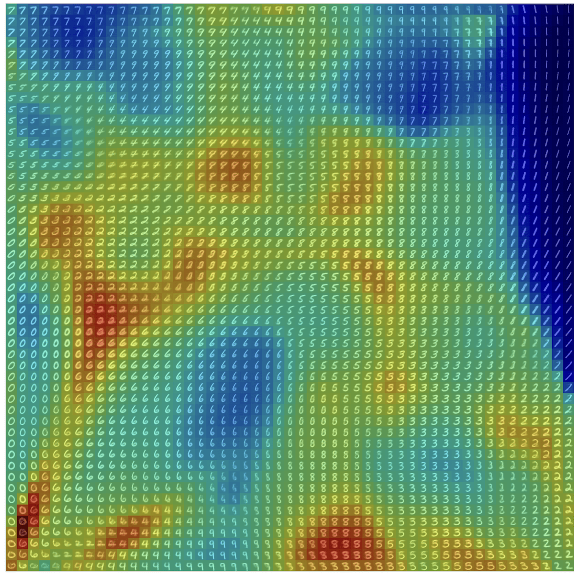
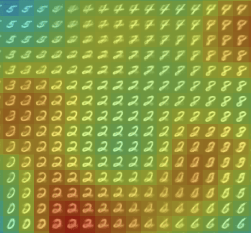
\(R(\tilde{x})\)
Example 2: priors for images
Learned Proximal Networks
\(R(\tilde{x})\)
x^{t+1} = \text{prox}_{\hat R} \left(x^t - \eta A^T(Ax^t - y)\right)
\hat x = \arg\min_x \frac 12 \| y - A x \|^2_2 + \hat{R}(x)
Learned Proximal Networks
via
Convergence Guarantees
Theorem (PGD with Learned Proximal Networks)
x^{t+1} = \text{prox}_{\hat R} \left(x^t - \eta A^T(Ax^t - y)\right)
\hat x = \arg\min_x \frac 12 \| y - A x \|^2_2 + \hat{R}(x)
Let \(f_\theta = \text{prox}_{\hat{R}} {\color{grey}\text{ with } \alpha>0}, \text{ and } 0<\eta<1/\sigma_{\max}(A) \) with smooth activations
\text{Then } \exists x^* : \lim_{k\to\infty} x^t = x^* \text{ and }
f_\theta(x^* - \eta A^T(Ax^*-y)) = x^*
(Analogous results hold for ADMM)
Learned Proximal Networks
Convergence guarantees for PnP
Fang, Buchanan & S. What's in a Prior? Learned Proximal Networks for Inverse Problems. ICLR 2024.
Learned Proximal Networks
\hat x = \arg\min_x \frac 12 \| y - A x \|^2_2 + \hat{R}(x)
What did my model learn?
PART I
Inverse Problems
PART II
Image Classification
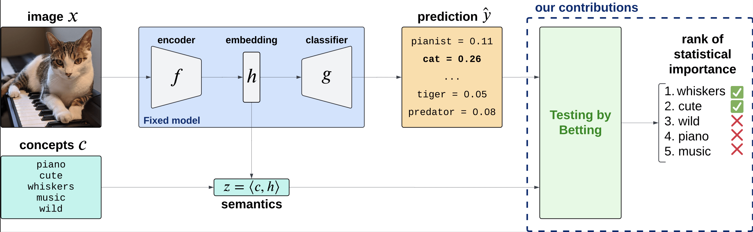
Interpretability in Image Classification
\((X,Y) \in \mathcal X \times \mathcal Y\)
\((X,Y) \sim P_{X,Y}\)
\(\hat{Y} = f(X) : \mathcal X \to \mathcal Y\)
Setting:

-
What features are important for this prediction?
-
What does importance mean, exactly?
Is the piano important for \(\hat Y = \text{cat}\)?
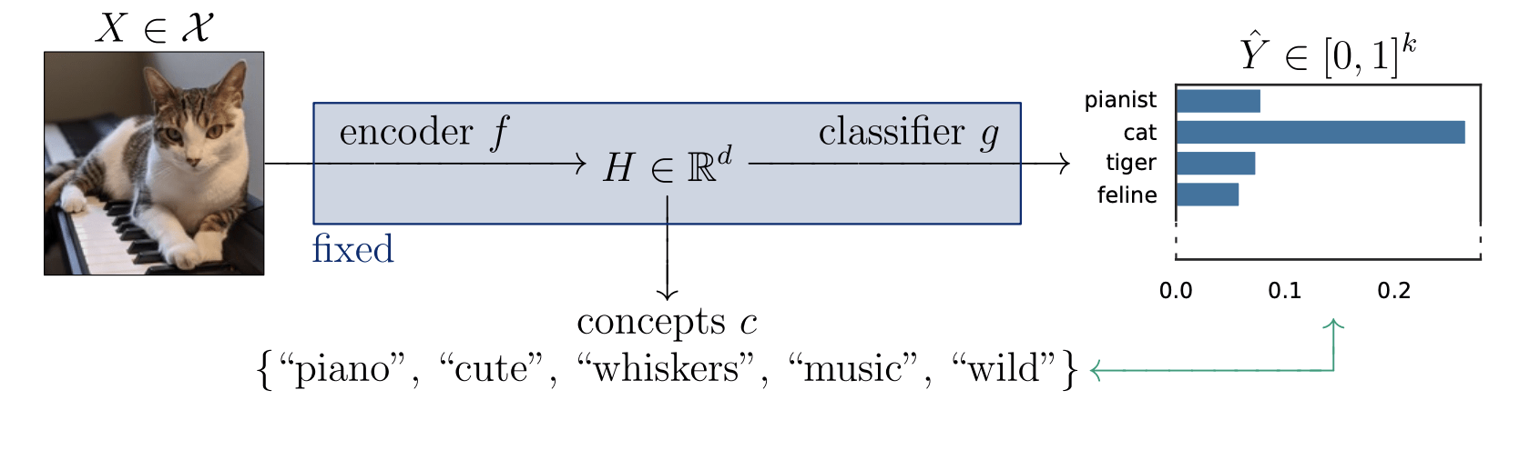
Semantic Interpretability of classifiers
How can we explain black-box predictors with semantic features?
Is the piano important for \(\hat Y = \text{cat}\), given that there is a cute mammal in the image?
Is the piano important for \(\hat Y = \text{cat}\)?
Semantic Interpretability of classifiers
How can we explain black-box predictors with semantic features?
Is the piano important for \(\hat Y = \text{cat}\), given that there is a cute mammal in the image?
Post-hoc Interpretability Methods
Interpretable by
construction
Semantic Interpretability of classifiers
Concept Bank: \(C = [c_1, c_2, \dots, c_m] \in \mathbb R^{d\times m}\)
Embeddings: \(H = f(X) \in \mathbb R^d\)
Semantics: \(Z = C^\top H \in \mathbb R^m\)
Concept Bank: \(C = [c_1, c_2, \dots, c_m] \in \mathbb R^{d\times m}\)
Concept Activation Vectors
(Kim et al, 2018)
\(c_\text{cute}\)
Semantic Interpretability of classifiers
Vision-language models
(CLIP, BLIP, etc... )
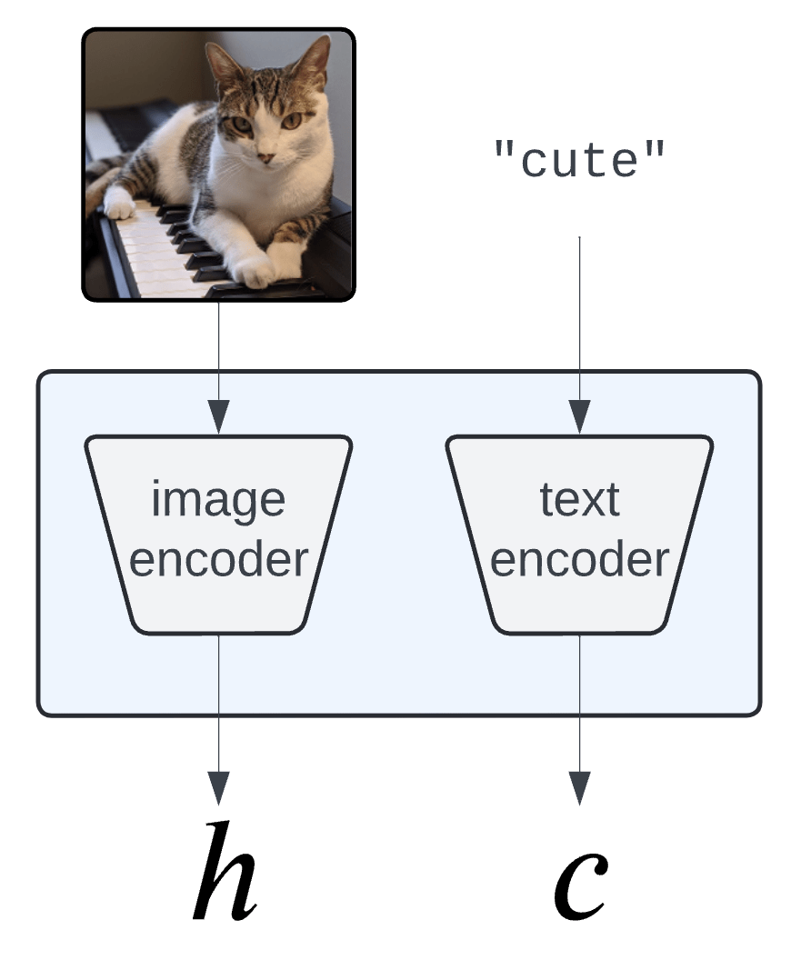
Semantic Interpretability of classifiers
[Bhalla et al, "Splice", 2024]
Concept Bottleneck Models (CMBs)
[Koh et al '20, Yang et al '23, Yuan et al '22 ]
- Need to engineer a (large) concept bank
- Performance hit w.r.t. original predictor
\(\tilde{Y} = \hat w^\top Z\)
\(\hat w_j\) is the importance of the \(j^{th}\) concept
Desiderata
- Fixed original predictor (post-hoc)
- Global and local importance notions
- Testing for any concepts (no need for large concept banks)
- Precise testing with guarantees (Type 1 error/FDR control)
Precise notions of semantic importance
\(C = \{\text{``cute''}, \text{``whiskers''}, \dots \}\)
Global Importance
\(H^G_{0,j} : \hat{Y} \perp\!\!\!\perp Z_j \)
Global Conditional Importance
\(H^{GC}_{0,j} : \hat{Y} \perp\!\!\!\perp Z_j | Z_{-j}\)
Precise notions of semantic importance
Global Importance
\(C = \{\text{``cute''}, \text{``whiskers''}, \dots \}\)
\(H^G_{0,j} : g(f(X)) \perp\!\!\!\perp c_j^\top f(X) \)
Global Conditional Importance
\(H^{GC}_{0,j} : g(f(X)) \perp\!\!\!\perp c_j^\top f(X) | C_{-j}^\top f(X)\)
\(H^G_{0,j} : \hat{Y} \perp\!\!\!\perp Z_j \)
\(H^{GC}_{0,j} : \hat{Y} \perp\!\!\!\perp Z_j | Z_{-j}\)
Precise notions of semantic importance
"The classifier (its distribution) does not change if we condition
on concepts \(S\) vs on concepts \(S\cup\{j\} \)"
\(C = \{\text{``cute''}, \text{``whiskers''}, \dots \}\)
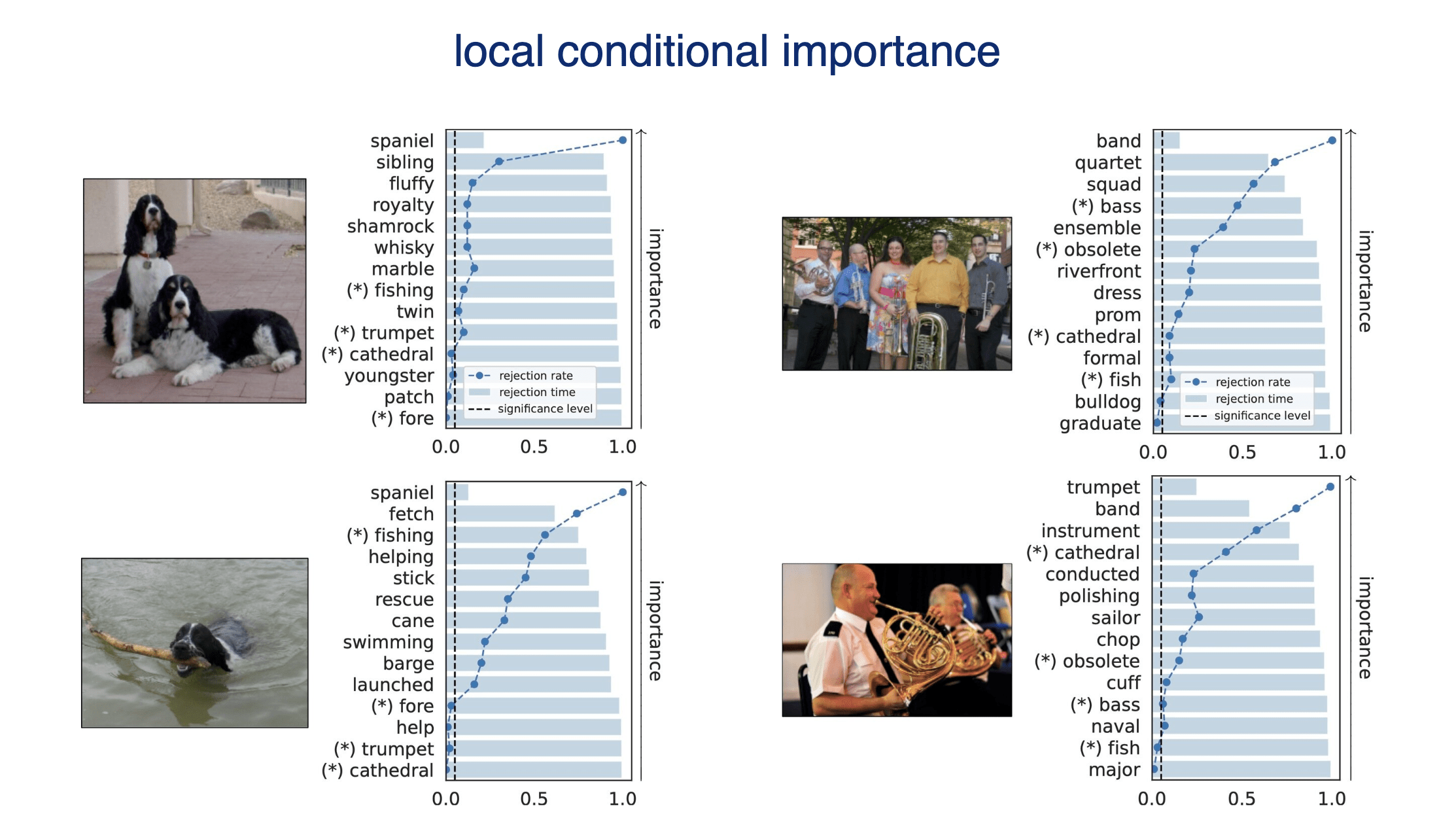
Local Conditional Importance
Tightly related to Shapley values
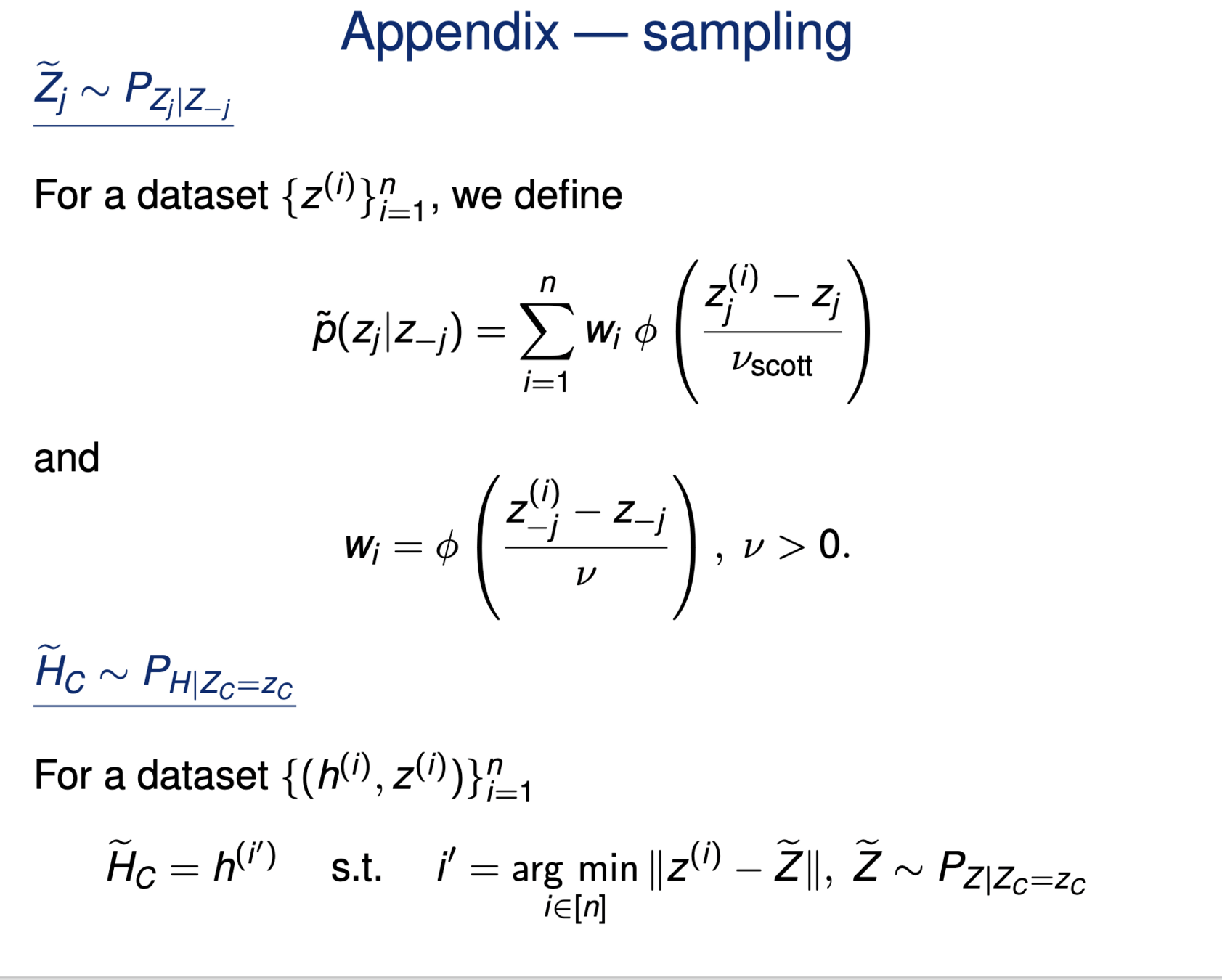
\[H^{j,S}_0:~ g({\tilde H_{S \cup \{j\}}}) \overset{d}{=} g(\tilde H_S), \qquad \tilde H_S \sim P_{H|Z_S = C_S^\top f(x)} \]
[Teneggi et al, The Shapley Value Meets Conditional Independence Testing, 2023]
Precise notions of semantic importance
"The classifier (its distribution) does not change if we condition
on concepts \(S\) vs on concepts \(S\cup\{j\} \)"
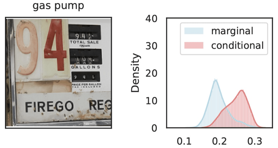

\(\hat{Y}_\text{gas pump}\)
\(Z_S\cup Z_{j}\)
\(Z_{S}\)
\(Z_j=\)
Local Conditional Importance
\[H^{j,S}_0:~ g({\tilde H_{S \cup \{j\}}}) \overset{d}{=} g(\tilde H_S), \qquad \tilde H_S \sim P_{H|Z_S = C_S^\top f(x)} \]
Precise notions of semantic importance
"The classifier (its distribution) does not change if we condition
on concepts \(S\) vs on concepts \(S\cup\{j\} \)"

\(\hat{Y}_\text{gas pump}\)
\(\hat{Y}_\text{gas pump}\)
\(Z_S\cup Z_{j}\)
\(Z_{S}\)
\(Z_S\cup Z_{j}\)
\(Z_{S}\)
Local Conditional Importance
\(Z_j=\)
\(Z_j=\)
\[H^{j,S}_0:~ g({\tilde H_{S \cup \{j\}}}) \overset{d}{=} g(\tilde H_S), \qquad \tilde H_S \sim P_{H|Z_S = C_S^\top f(x)} \]
Testing by betting
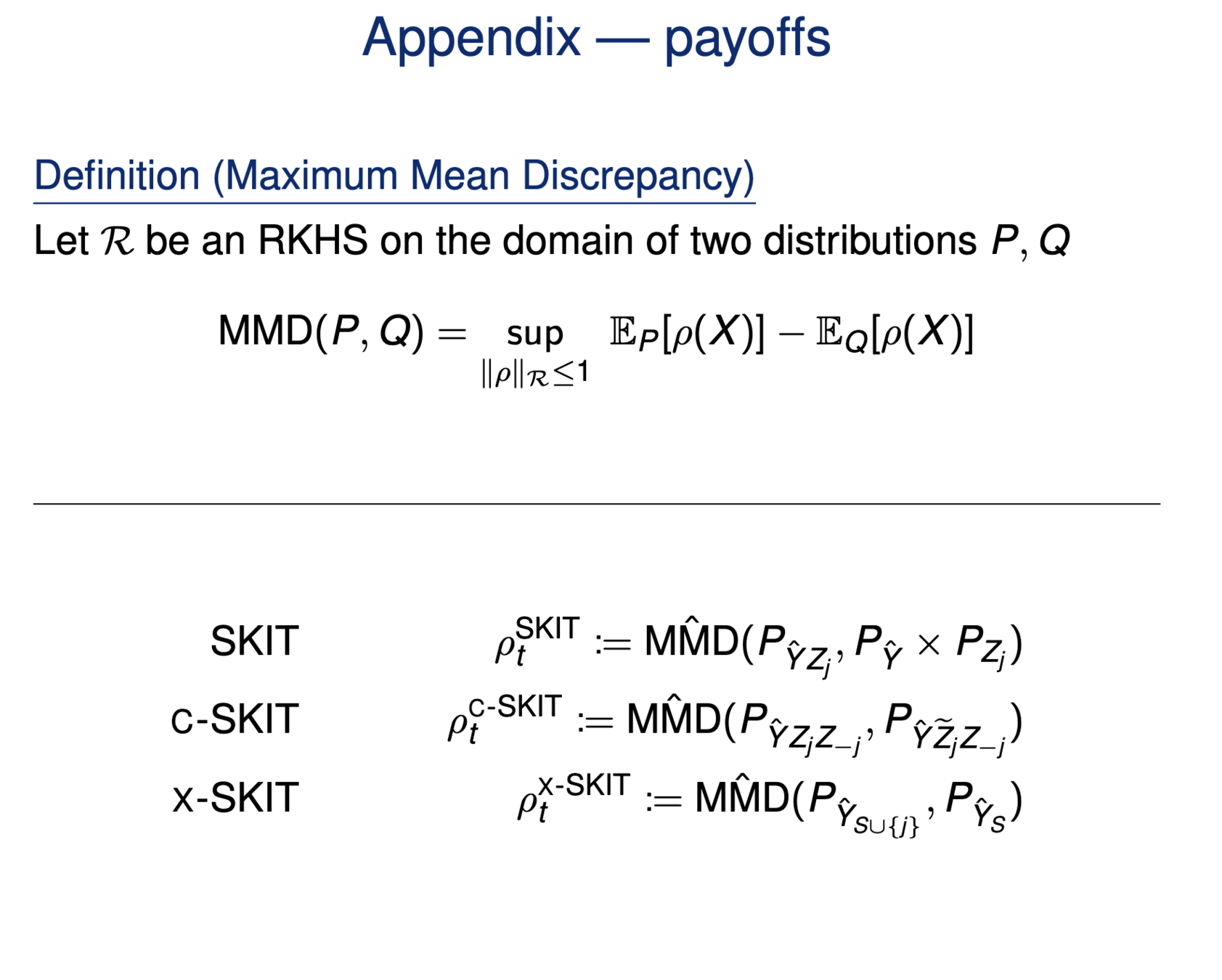
\(H^G_{0,j} : \hat{Y} \perp\!\!\!\perp Z_j \iff P_{\hat{Y},Z_j} = P_{\hat{Y}} \times P_{Z_j}\)
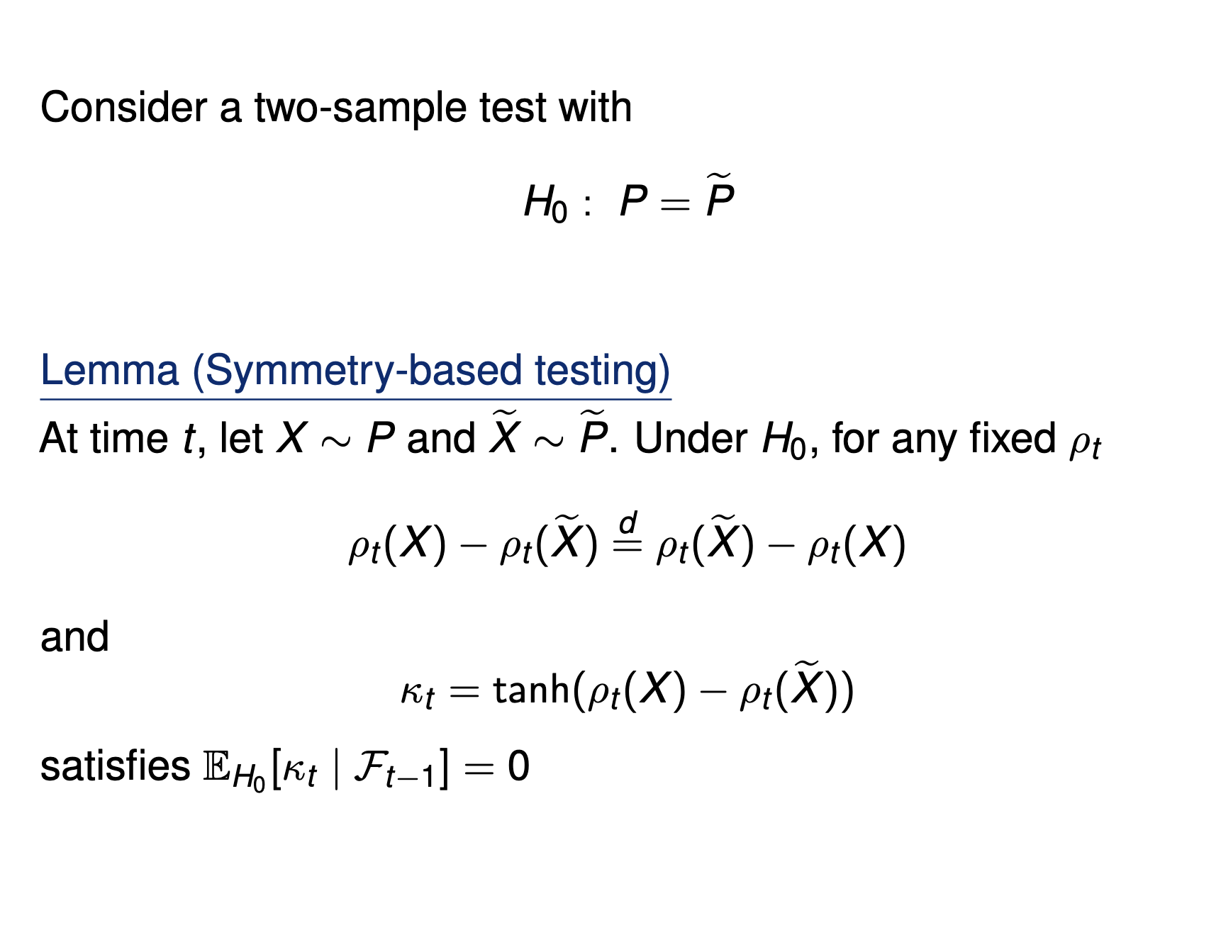
Testing importance via two-sample tests
\(H^{GC}_{0,j} : \hat{Y} \perp\!\!\!\perp Z_j | Z_{-j} \iff P_{\hat{Y}Z_jZ_{-j}} = P_{\hat{Y}\tilde{Z}_j{Z_{-j}}}\)
\(\tilde{Z_j} \sim P_{Z_j|Z_{-j}}\)
[Shaer et al, 2023]
[Teneggi et al, 2023]
\[H^{j,S}_0:~ g({\tilde H_{S \cup \{j\}}}) \overset{d}{=} g(\tilde H_S), \qquad \tilde H_S \sim P_{H|Z_S = C_S^\top f(x)} \]
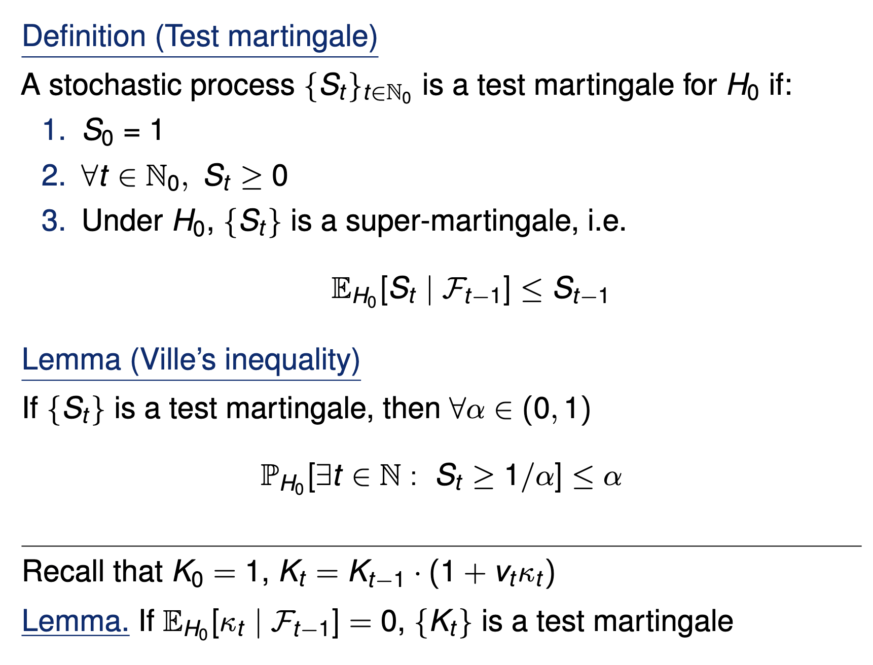
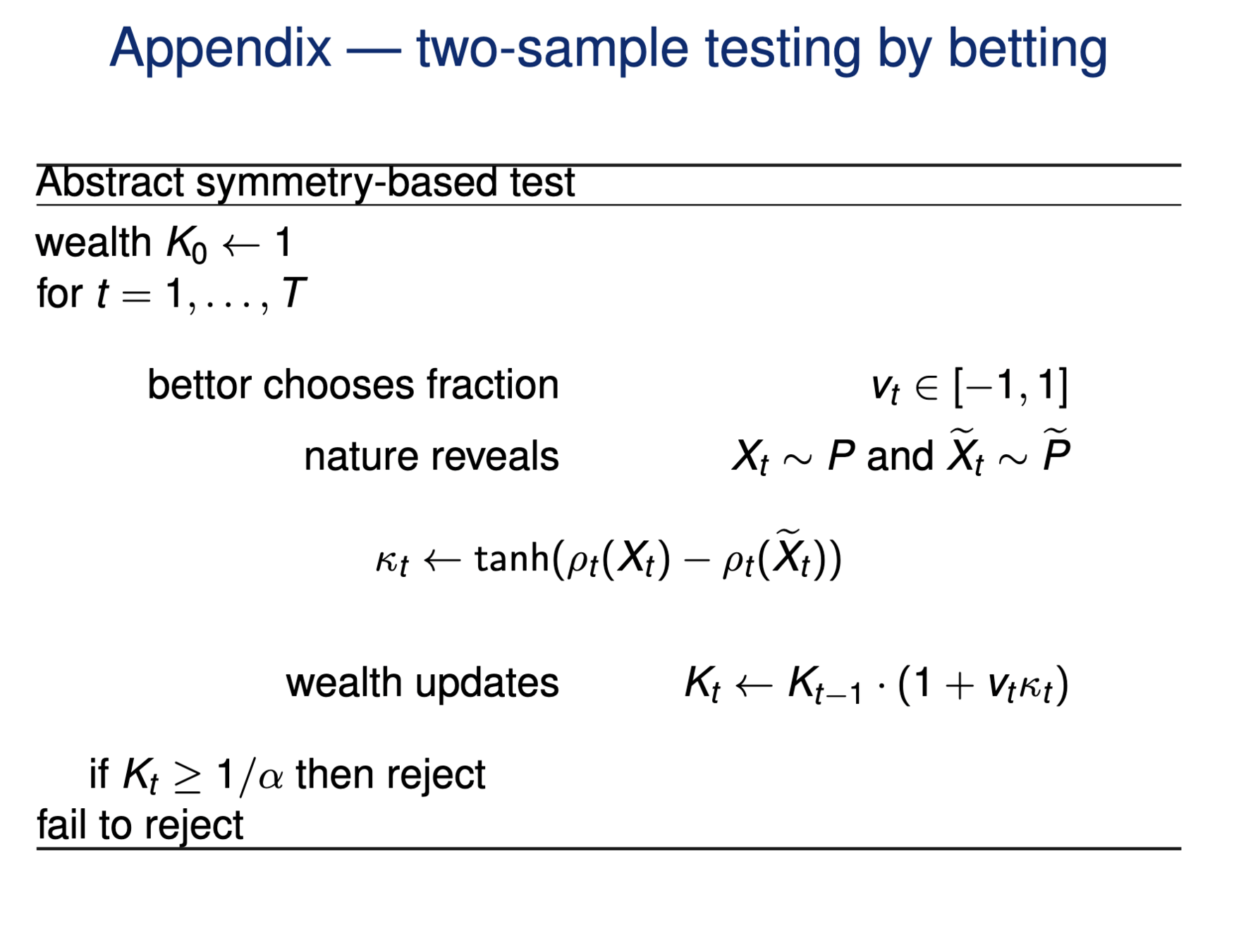
Testing by betting
[Shaer et al. 2023, Shekhar and Ramdas 2023 ]
Goal: Test a null hypothesis \(H_0\) at significance level \(\alpha\)
Standard testing by p-values
Collect data, then test, and reject if \(p \leq \alpha\)
Online testing by e-values
Any-time valid inference, monitor online and reject when \(e\geq 1/\alpha\)
- Consider a wealth process
\(K_0 = 1;\)
\(\text{for}~ t = 1, \dots \\ \)
Reject \(H_0\) when \(K_t \geq 1/\alpha\)
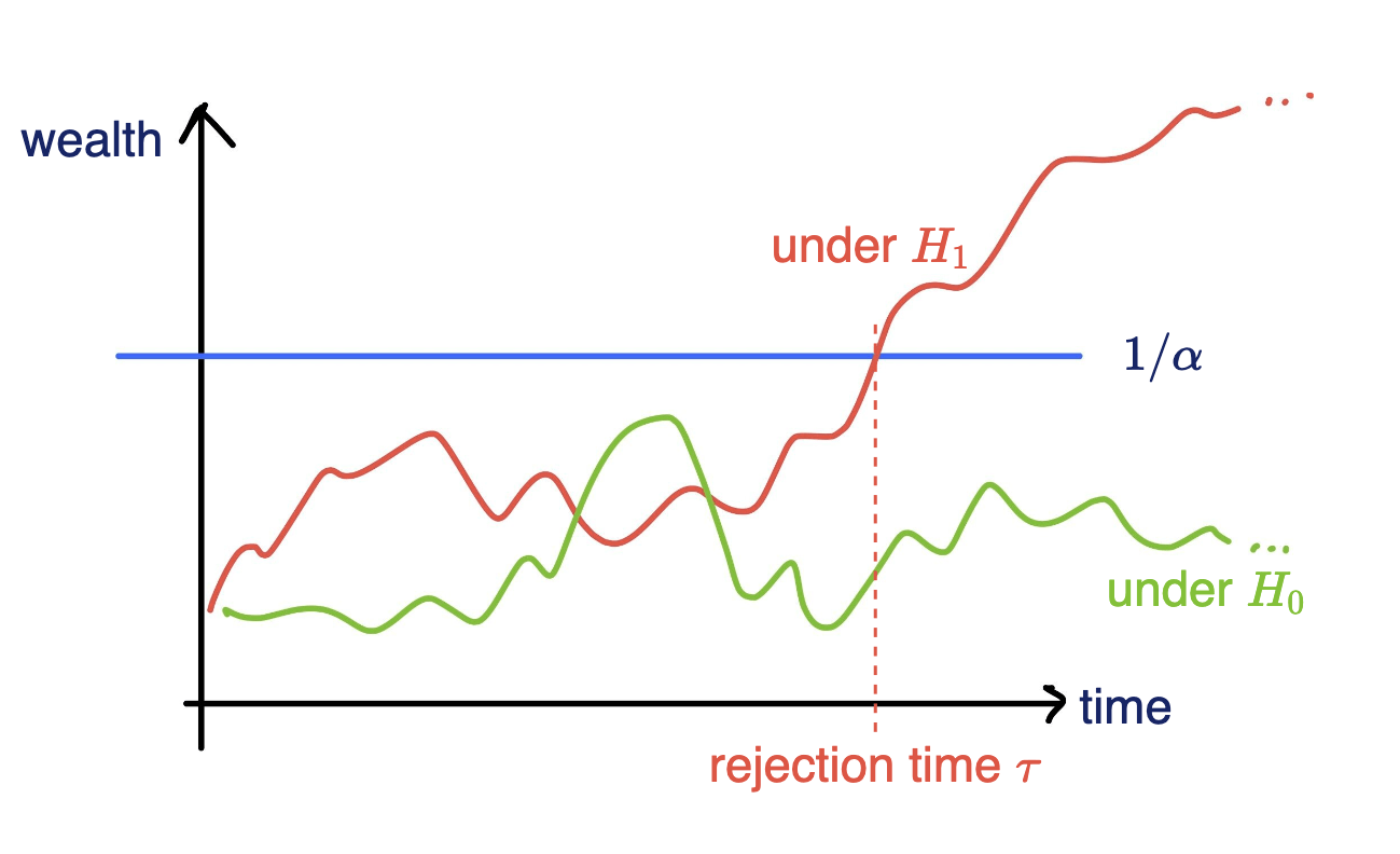
Online testing by e-values
[Shaer et al. 2023, Shekhar and Ramdas 2023 ]
Fair game: \(~~\mathbb E_{H_0}[\kappa_t | \text{Everything seen}_{t-1}] = 0\)
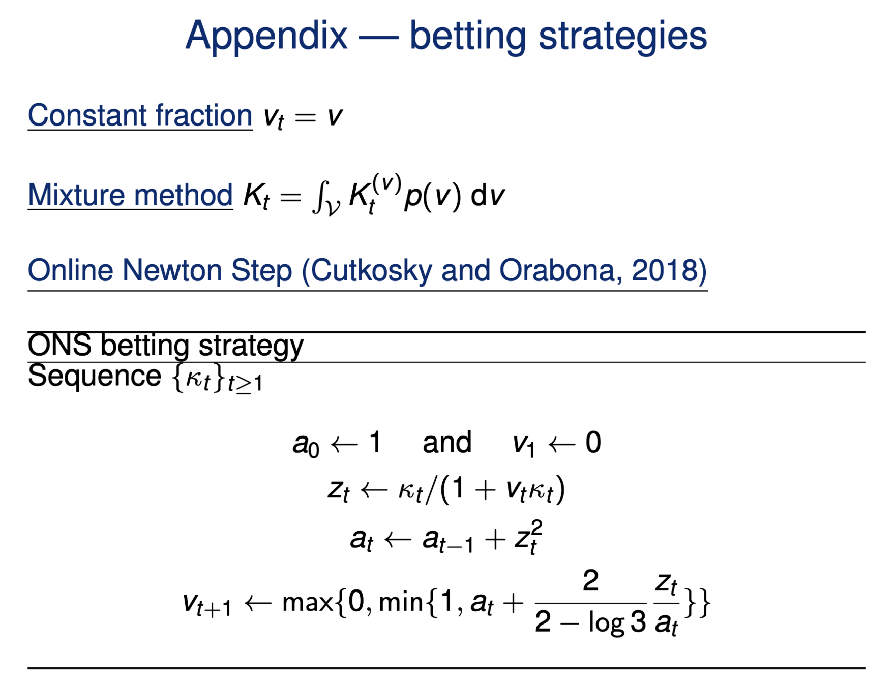
\(v_t \in (0,1):\) betting fraction
\(\kappa_t \in [-1,1]\) payoff
\( K_t = K_{t-1}(1+\kappa_t v_t)\)
Testing by betting via SKIT (Podkopaev et al., 2023)
Online testing by e-values
\(v_t \in (0,1):\) betting fraction
\(H_0: ~ P = Q\)
\(\kappa_t = \text{tahn}({\color{teal}\rho(X_t)} - {\color{teal}\rho(Y_t)})\)
Payoff function
\({\color{black}\text{MMD}(P,Q)} = \underset{\rho \in R : \|\rho\|_\mathcal{R} \leq 1}{\sup} \mathbb E_P [\rho(X)] - \mathbb E_Q [\rho(Y)]\)
\({\color{teal}\rho} = \underset{\rho\in \mathcal R:\|\rho\|_\mathcal R\leq 1}{\arg\sup} ~\mathbb E_P [\rho(X)] - \mathbb E_Q[\rho(Y)]\)
\( K_t = K_{t-1}(1+\kappa_t v_t)\)
Data efficient
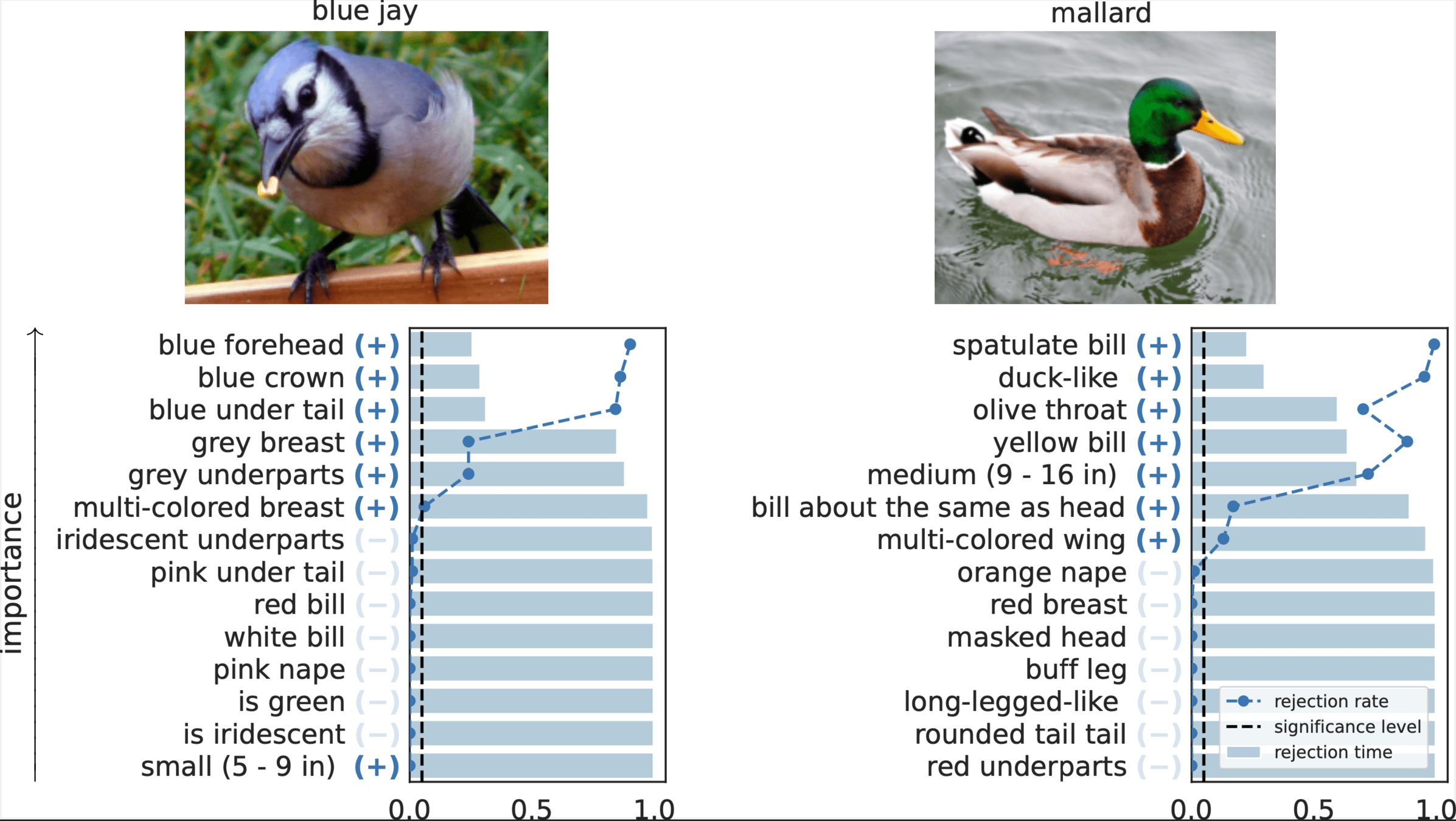
Rank induced by rejection time
Testing by betting via SKIT (Podkopaev et al., 2023)

rejection time
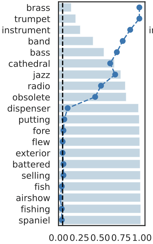

rejection rate
Important Semantic Concepts
(Reject \(H_0\))

Unimportant Semantic Concepts
(fail to reject \(H_0\))
Results
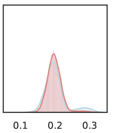
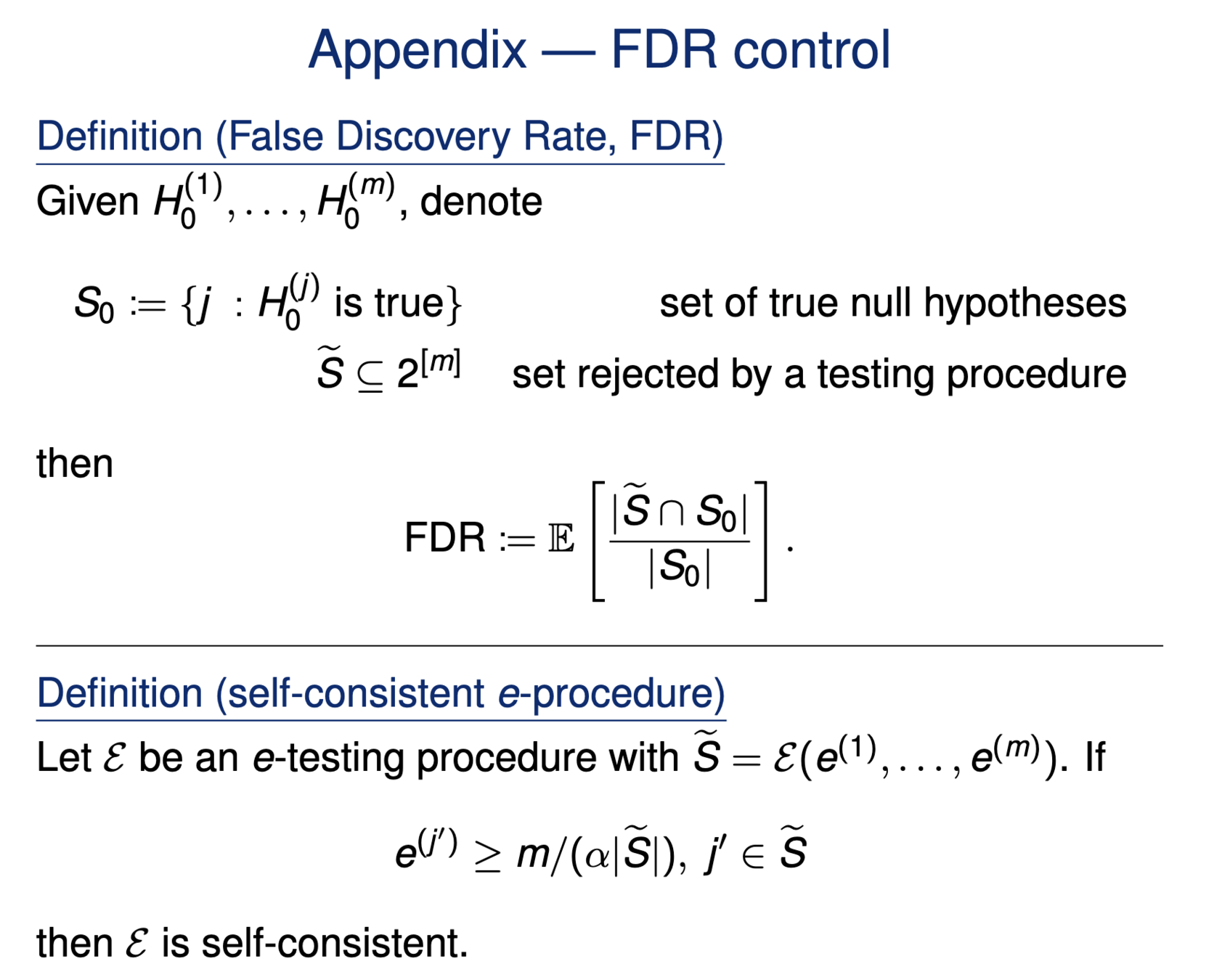
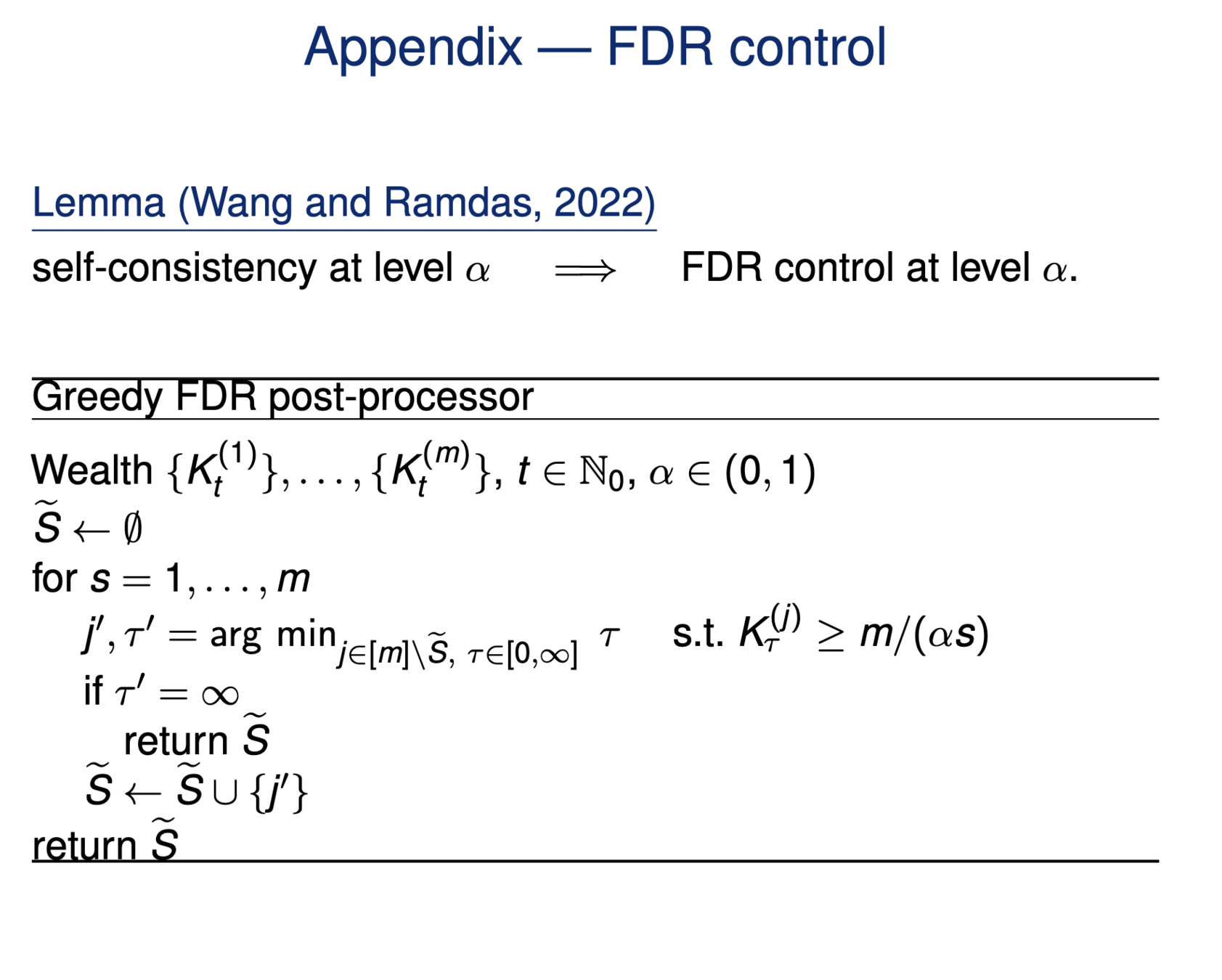
Type 1 error control
False discovery rate control
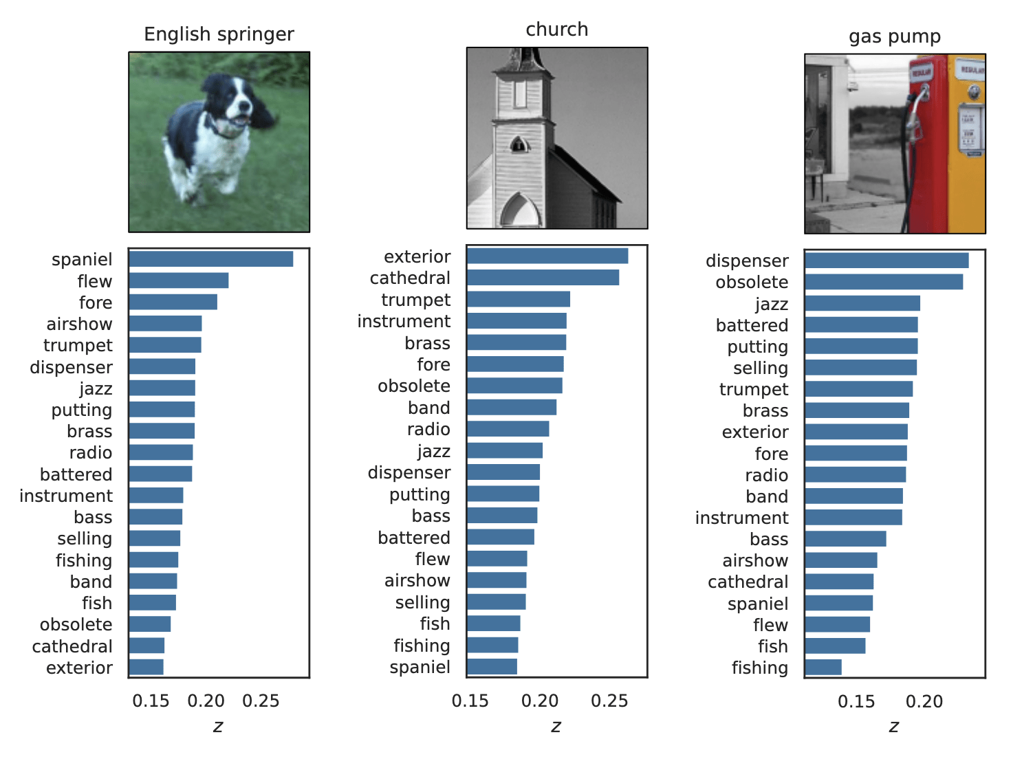
Results: CUB dataset
Results: Imagenette
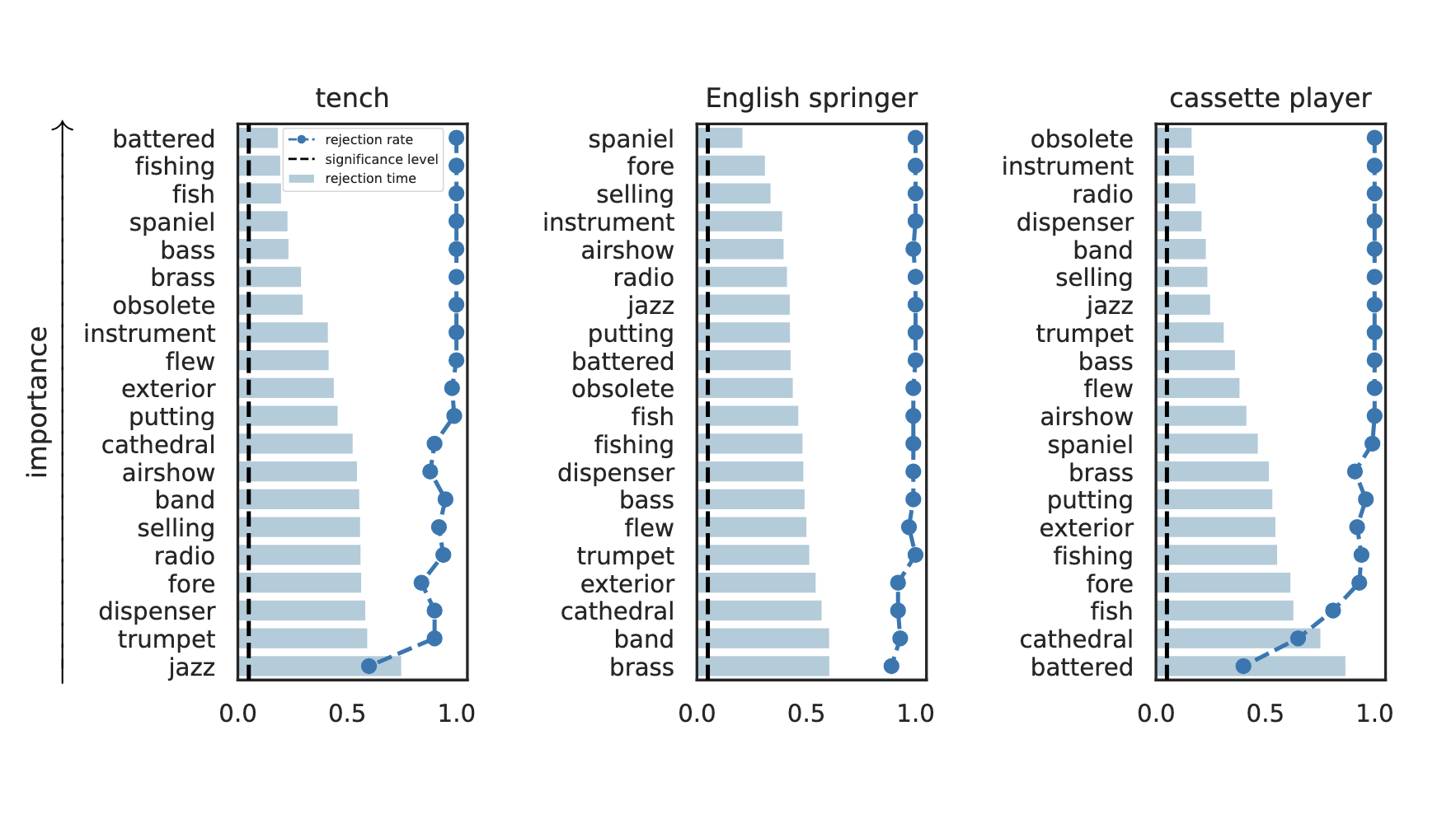
Global Importance
Results: Imagenette
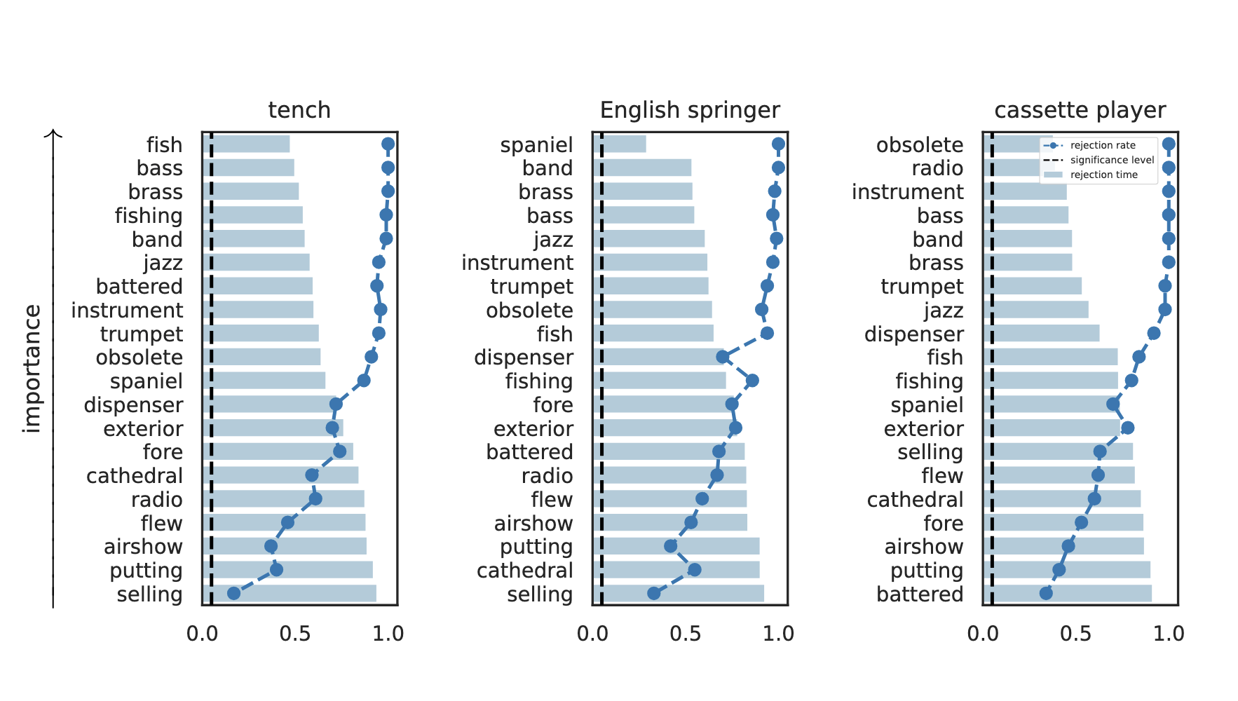
Global Conditional Importance
Results: Imagenette

Results: Imagenette
Results: Imagenette
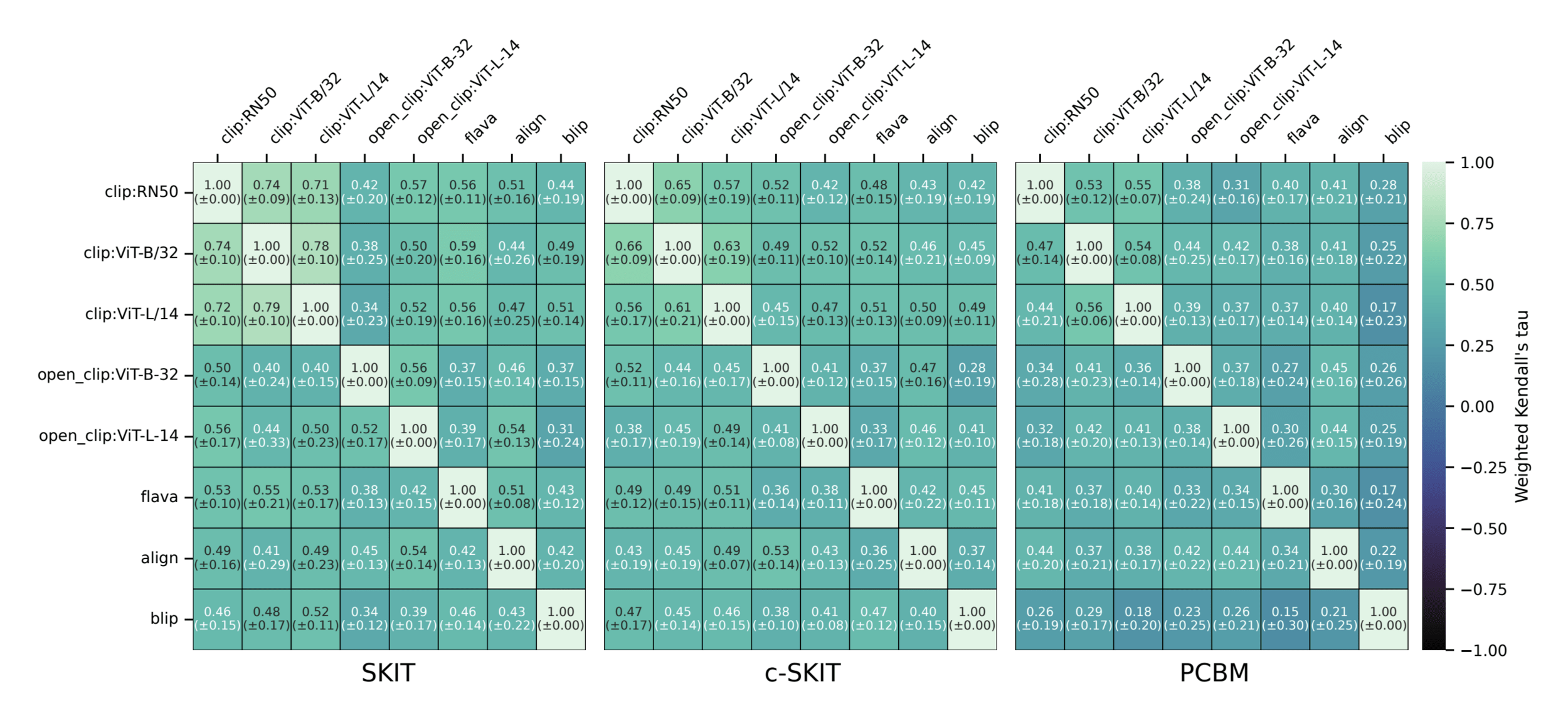
Semantic comparison of vision-language models
-
Exciting open problems to making AI tools safe, trustworthy and interpretable
-
Importance in clear definitions and guarantees
Concluding Remarks
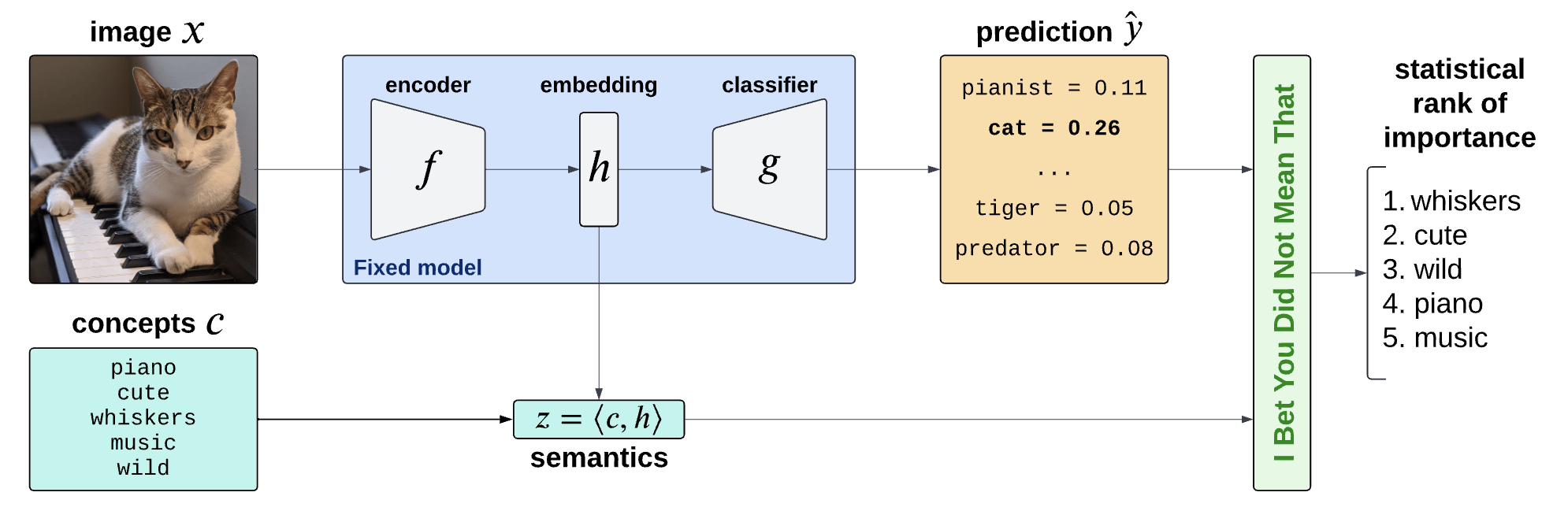
* Fang, Z., Buchanan, S., & J.S. (2023). What's in a Prior? Learned Proximal Networks for Inverse Problems. International Conference on Learning Representations (ICLR 2024).


* Teneggi, J. and J.S. I Bet You Did Not Mean That: Testing Semantic Importance via Betting. NeurIPS 2024 (to appear).


...that's it!


Zhenghan Fang
JHU
Jacopo Teneggi
JHU
Beepul Bharti
JHU
Sam Buchanan
TTIC
Yaniv Romano
Technion
Appendix
\hat x = \arg\min_x \frac 12 \| y - A x \|^2_2 + \hat{R}(x)
Learned Proximal Networks
Convergence guarantees for PnP
x^{t+1} = f_\theta \left(x^t - \eta A^T(Ax^t - y)\right)
- [Sreehari et al., 2016; Sun et al., 2019; Chan, 2019; Teodoro et al., 2019]
Convergence of PnP for non-expansive denoisers. -
[Ryu et al, 2019]
Convergence for close to contractive operators - [Xu et al, 2020]
Convergence of Plug-and-Play priors with MMSE denoisers -
[Hurault et al., 2022]
Lipschitz-bounded denoisers
-
Sensitivity or Gradient-based perturbations
-
Shapley coefficients
-
Variational formulations
-
Counterfactual & causal explanations
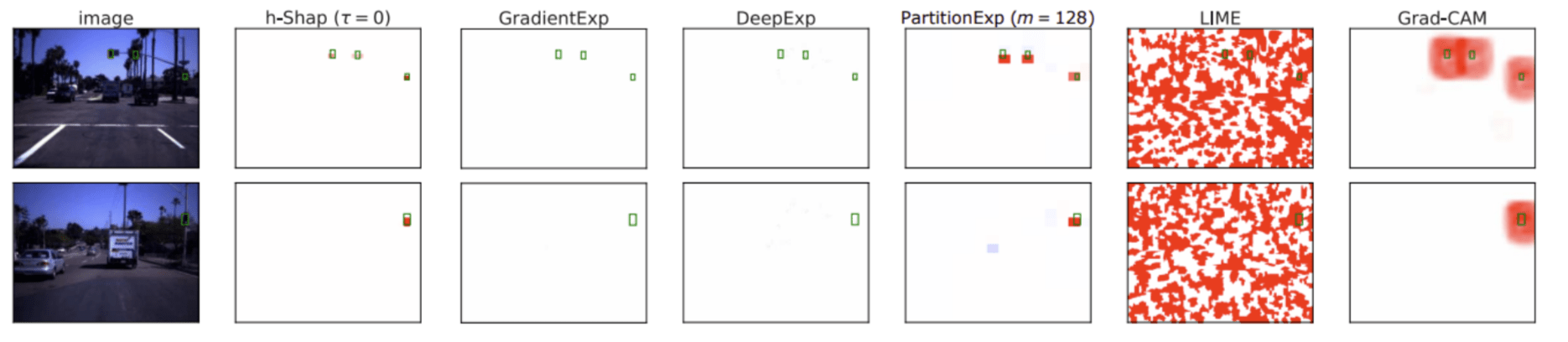
LIME [Ribeiro et al, '16], CAM [Zhou et al, '16], Grad-CAM [Selvaraju et al, '17]
Shap [Lundberg & Lee, '17], ...
RDE [Macdonald et al, '19], ...
[Sani et al, 2020] [Singla et al '19],..

Post-hoc Interpretability in Image Classification
efficiency
nullity
symmetry
exponential complexity
Lloyd S Shapley. A value for n-person games. Contributions to the Theory of Games, 2(28):307–317, 1953.
Let be an -person cooperative game with characteristic function
G = ([n],f)
n
f : \mathcal P([n]) \mapsto \mathbb R
How important is each player for the outcome of the game?
\displaystyle \phi_i = \sum_{S_j\subseteq [n]\setminus \{i\} } w_{S_j} \left[ f(S_j\cup \{i\}) - f(S_j) \right]
marginal contribution of player i with coalition S
Shapley values
\displaystyle \phi_i = \sum_{S_j\subseteq [n]\setminus \{i\}} w_j ~ \mathbb ~~ \left[ f(\tilde X_{S_j\cup \{i\}}) - f(\tilde X_{S_j}) \right]
Shap-Explanations
X \in \mathcal X \subset \mathbb R^n
Y\in \mathcal Y = \{0,1\}
inputs
responses
f:\mathcal X \to \mathcal Y
predictor
How important is feature \(x_i\) for \(f(x)\)?
x_{S_j}
\tilde{X}_{S_j}:
X_{S_j^c}
\(X_{S_j^c}\sim \mathcal D_{X_{S_j}={x_{S_j}}}\)
Scott Lundberg and Su-In Lee. A Unified Approach to Interpreting Model Predictions, NeurIPS , 2017
\displaystyle \phi_i = \sum_{S_j\subseteq [n]\setminus \{i\}} w_j ~ \mathbb E \left[ f(\tilde X_{S_j\cup \{i\}}) - f(\tilde X_{S_j}) \right]
Shap-Explanations
X \in \mathcal X \subset \mathbb R^n
Y\in \mathcal Y = \{0,1\}
inputs
responses
How important is feature \(x_i\) for \(f(x)\)?
x_{S_j}
\tilde{X}_{S_j}:
X_{S_j^c}
f:\mathcal X \to \mathcal Y
predictor
\(X_{S_j^c}\sim \mathcal D_{X_{S_j}={x_{S_j}}}\)
Scott Lundberg and Su-In Lee. A Unified Approach to Interpreting Model Predictions, NeurIPS , 2017
Question 2) What do these coefficients mean, really?
Precise notions of importance
Formal Feature Importance
H_{0,S}:~ X_S \perp\!\!\!\perp Y | X_{[n]\setminus S}
[Candes et al, 2018]
Question 2) What do these coefficients mean, really?
Precise notions of importance

XRT: eXplanation Randomization Test
returns a \(\hat{p}_{i,S}\) for the test above
\text{reject} ~\Rightarrow~ i=2 \text{: important}
H^0_{i=2,S=\{1,3,4\}}
i=1
i=2
i=3
i=4
How do we test?
\text{For any } S \subseteq [n]\setminus \{{\color{Red}i}\}, \text{ and a sample } x\sim \mathcal p_X
H^0_{{\color{red}i},S}:~ (f(\tilde X_{S\cup \{{\color{red}i}\}}) ) \overset{d}{=} (f(\tilde X_{S}) )
Local Feature Importance
Precise notions of importance
Local Feature Importance
\text{For any } S \subseteq [n]\setminus \{{\color{Red}i}\}, \text{ and a sample } x\sim \mathcal D_X
H^0_{{\color{red}i},S}:~ (f(\tilde X_{S\cup \{{\color{red}i}\}}) ) \overset{d}{=} (f(\tilde X_{S}) )
\gamma_{i,S}
\displaystyle \phi_{\color{red}i}(x) = \sum_{S\subseteq [n]\setminus \{{\color{red}i}\}} w_{S} ~ \mathbb E \left[ f(\tilde X_{S\cup \{{\color{red}i}\}}) - f(\tilde X_S) \right]
Given the Shapley coefficient of any feature
Then
p_{i,S}
and the (expected) p-value obtained for , i.e. ,
H^0_{i,S}
Theorem:
p_{i,S} \leq 1 - \gamma_{i,S}.
i\in[n],
Teneggi, Bharti, Romano, and S. "SHAP-XRT: The Shapley Value Meets Conditional Independence Testing." TMLR (2023).
Question 3)
How to go beyond input-features explanations?
Shap-Explanations
Question 1)
Can we resolve the computational bottleneck (and when) ?
Question 2)
What do these coefficients mean, really?
Question 3)
How to go beyond input-features explanations?

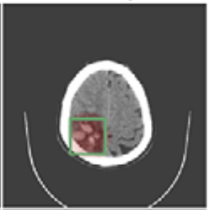
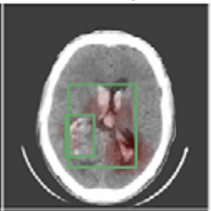
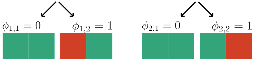
We focus on data with certain structure:
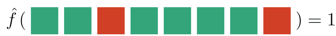
f\huge(
{\huge)} = 0
{f}\huge(
{\huge)} = 1
{f}\huge(
{\huge)} = 0
Example:
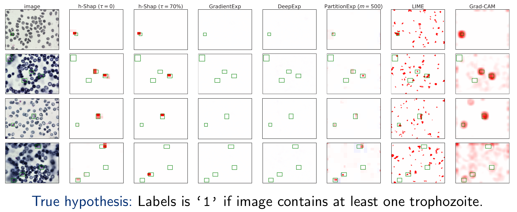
f(x) = 1
if contains a sick cell
x

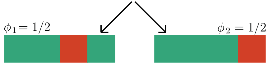
Hierarchical Shap (h-Shap)
\text{\textbf{Assumption 1:}}~ f(x) = 1 \Leftrightarrow \exist~ i: f(\tilde X_i) = 1
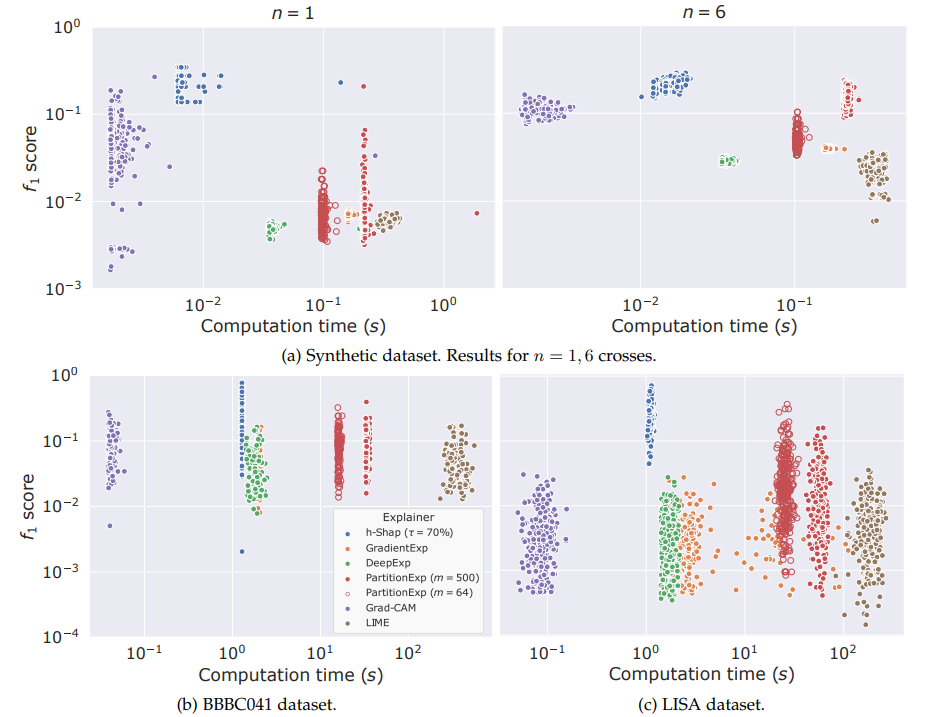
Question 1) Can we resolve the computational bottleneck (and when) ?
Theorem (informal)
-
hierarchical Shap runs in linear time
-
Under A1, h-Shap \(\to\) Shapley
\mathcal O(2^\gamma k \log n)
[Teneggi, Luster & S., IEEE TPAMI, 2022]

We focus on data with certain structure:
Hierarchical Shap (h-Shap)
\text{\textbf{Assumption 1:}}~ f(x) = 1 \Leftrightarrow \exist~ i: f(\tilde X_i) = 1
Question 1) Can we resolve the computational bottleneck (and when) ?
Theorem (informal)
-
h-Shap runs in linear time
-
Under A1, h-Shap \(\to\) Shapley
\mathcal O(2^\gamma k \log n)
Fast hierarchical games for image explanations, Teneggi, Luster & S., IEEE Transactions on Pattern Analysis and Machine Intelligence, 2022
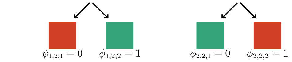
\gamma = 2
We focus on data with certain structure:
\text{\textbf{Assumption 1:}}~ f(x) = 1 \Leftrightarrow \exist~ i: f(\tilde X_i) = 1
Theorem (informal)
-
h-Shap runs in linear time
-
Under A1, h-Shap \(\to\) Shapley
\mathcal O(2^\gamma k \log n)
Hierarchical Shap (h-Shap)
Hierarchical Shap (h-Shap)
Fast hierarchical games for image explanations, Teneggi, Luster & Sulam, IEEE Transactions on Pattern Analysis and Machine Intelligence, 2022
Hierarchical Shap (h-Shap)
f \approx \mathbb E[Y|X=x]
X \in \mathcal X \subset \mathbb R^n
Y\in \mathcal Y = \{0,1\}
inputs
responses
f:\mathcal X \to \mathcal Y
\text{For any}~ S \subset [n],~ \text{and a sample } { x} \newline
\text{ define }\tilde{X}_S = [{x_S},X_{S^c}], \text{ where } X_{S^c}\sim \mathcal D_{X_S={x_S}}
predictor
Shap-Explanations
x_S
x:
x_{S^c}
\tilde{X}_S:
Shap-Explanations
x_S
x

\tilde{X}_S
f \approx \mathbb E[Y|X=x]
X \in \mathcal X \subset \mathbb R^n
Y\in \mathcal Y = \{0,1\}
inputs
responses
f:\mathcal X \to \mathcal Y
\text{For any}~ S \subset [n],~ \text{and a sample } { x} \newline
\text{ define }\tilde{X}_S = [{x_S},X_{S^c}], \text{ where } X_{S^c}\sim \mathcal D_{X_S={x_S}}
predictor
\displaystyle \phi_i = \sum_{S_j\subseteq [n]\setminus \{i\}} w_j ~ \mathbb E \left[ f(\tilde X_{S_j\cup \{i\}}) - f(\tilde X_{S_j}) \right]
Scott Lundberg and Su-In Lee. A Unified Approach to Interpreting Model Predictions, NeurIPS , 2017
efficiency
nullity
symmetry
exponential complexity
Shap-Explanations
f \approx \mathbb E[Y|X=x]
X \in \mathcal X \subset \mathbb R^n
Y\in \mathcal Y = \{0,1\}
inputs
responses
f:\mathcal X \to \mathcal Y
\text{For any}~ S \subset [n],~ \text{and a sample } { x} \newline
\text{ define }\tilde{X}_S = [{x_S},X_{S^c}], \text{ where } X_{S^c}\sim \mathcal D_{X_S={x_S}}
predictor
\gamma = 2
We focus on data with certain structure:
\text{\textbf{Assumption 1:}}~ f^*(x) = 1 \Leftrightarrow \exist~ i: f^*(\tilde X_i) = 1
Theorem (informal)
-
h-Shap runs in linear time
-
Under A1, h-Shap \(\to\) Shapley
\mathcal O(2^\gamma k \log n)
Hierarchical Shap (h-Shap)
Hierarchical Shap (h-Shap)
Teneggi, Luster & S. Fast hierarchical games for image explanations, IEEE Transactions on Pattern Analysis and Machine Intelligence, 2022Hierarchical Shap (h-Shap)
What has my model learned? UMich
By Jeremias Sulam


