Introduction to neural networks

Kolmogorov

Every continuous function of several variables defined on the unit cube can be represented as a superposition of continuous functions of one variable and the operation of addition (1957).

f(x_1,x_2, \ldots, x_n) = \sum\limits_{i=1}^{2n+1}f_i(\sum\limits_{j=1}^{n}\phi_{i,j}(x_j))

f(x_1,x_2, \ldots, x_n) = \sum\limits_{i=1}^{2n+1}f_i(\sum\limits_{j=1}^{n}\phi_{i,j}(x_j))

Thus, it is as if there are no functions of several variables at all. There are only simple combinations of functions of one variable.

f_1

f_1

f_i

f_i

f_{2n+1}

f_{2n+1}

f(x_1,x_2, \ldots, x_n) = \sum\limits_{i=1}^{2n+1}f_i(\sum\limits_{j=1}^{n}\phi_{i,j}(x_j))

f(x_1,x_2, \ldots, x_n) = \sum\limits_{i=1}^{2n+1}f_i(\sum\limits_{j=1}^{n}\phi_{i,j}(x_j))

x_1

x_1

x_2

x_2

x_n

x_n

\phi_{1,n}

\phi_{1,n}

\phi_{2n+1,n}

\phi_{2n+1,n}

\phi_{2n+1,1}

\phi_{2n+1,1}

\phi_{1,1}

\phi_{1,1}

\phi_{1,2}

\phi_{1,2}

\phi_{2n+1,2}

\phi_{2n+1,2}

f

f

\Phi(x_1,x_2,\cdots,x_n) = \rho(\sum\limits_{i=1}^n a_i x_i+b)

\Phi(x_1,x_2,\cdots,x_n) = \rho(\sum\limits_{i=1}^n a_i x_i+b)

a_1

a_1

a_2

a_2

a_n

a_n

x_1

x_1

x_2

x_2

x_n

x_n

\mathbb{R}^n \stackrel{\Phi}{\rightarrow}\mathbb{R}^1

\mathbb{R}^n \stackrel{\Phi}{\rightarrow}\mathbb{R}^1

one ''hidden layer"
one "node"
"activation" rho
"threshold" b

\rho

\rho

Example Feedforward neural network (one "hidden" layer and one node)

\text{where } \rho(x):= \text{max}(0,x)

\text{where } \rho(x):= \text{max}(0,x)

Definition Feedforward neural network (cited from this paper) a.k.a. MLP or ReLu neural network. L-1 hidden layers.

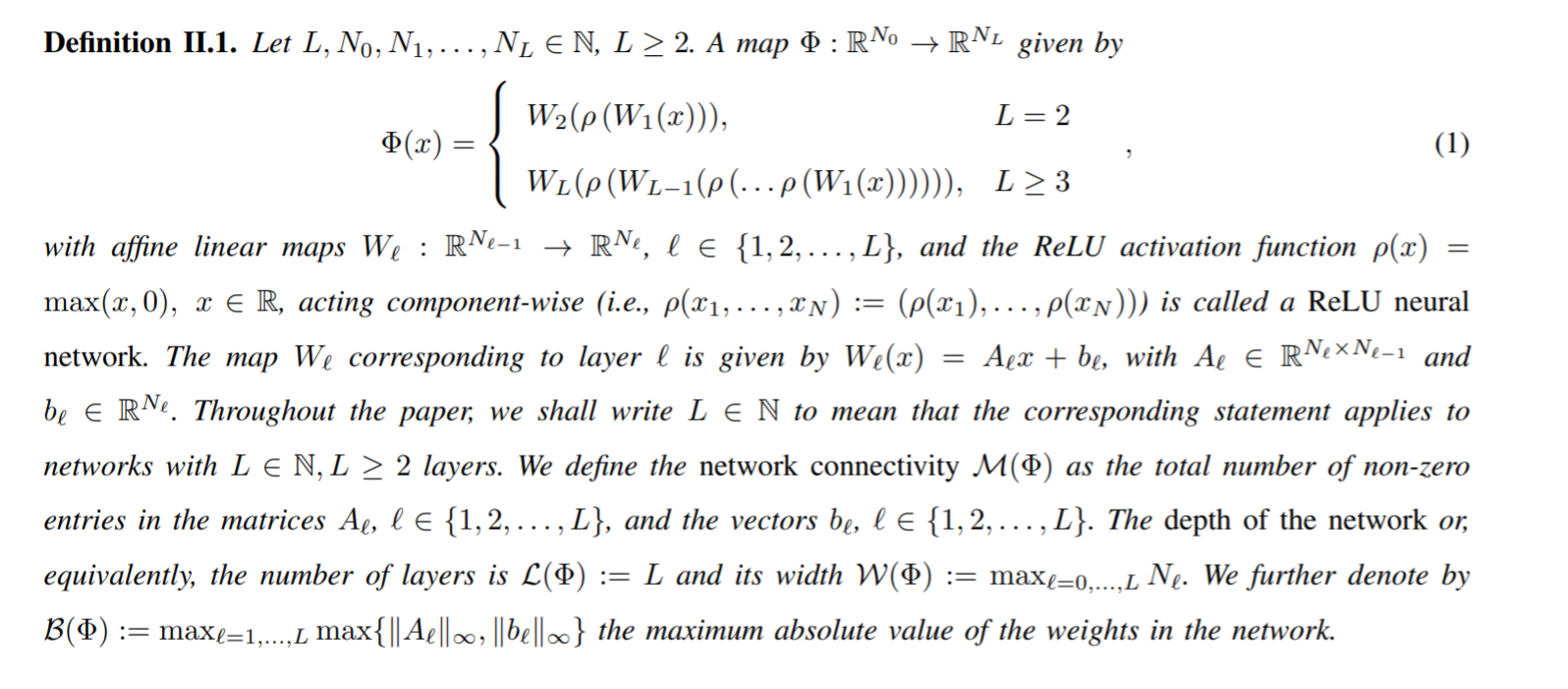
L=3,\\ N_0 = 4,\\ N_1 = 4,\\ N_2 = 7,\\ N_3 = 3

L=3,\\ N_0 = 4,\\ N_1 = 4,\\ N_2 = 7,\\ N_3 = 3

Here there are two hidden layers (ReLu maps), 3 layers (affine maps). The ReLu maps not displayed.

Image from https://www.doc.ic.ac.uk/~nuric/

Introduction to neural networks

QTM

Institute for quantitative theory and methods

Neural networks

Mathematical intuition

Definition

one ''hidden layer"

one "node"

"activation" rho

"threshold" b

Example Feedforward neural network (one "hidden" layer and one node)

Definition Feedforward neural network (cited from this paper) a.k.a. MLP or ReLu neural network. L-1 hidden layers.

Thank you!

Introduction to neural networks

Introduction to neural networks

Jeremy Jacobson

Introduction to neural networks

QTM

Institute for quantitative theory and methods

Introduction to neural networks

More from Jeremy Jacobson